Introduction
Excel data tables are pretty sweet, right? They enable you to perform sensitivity analysis with minimal effort. (For those of you who haven’t dealt with Excel data tables before, here’s a quick primer). For those of you enamored with data tables, I’ve got bad news: you could be doing it better.
If you’re doing something quick ‘n’ dirty, Excel data tables are okay. For anything more complicated, or any analysis that will be a recurring piece of your project / presentation, you shouldn’t use them.
This article will show you a better way to perform sensitivity analysis - leading to clearer, more auditable models.
Background Articles
This article will build off the prior two articles, so if you haven’t worked through those, please go to square 1.
Why not data tables?
Below is a summary of the main problems with data tables.
Hard-codes
Variables sensitized using Excel data tables must be hard-coded. Oftentimes, however, the variables that you want to sensitize in a data table are the same variables you would like to include in your cases (covered in the prior article - #2 in the list above).
In the short-run, this isn’t a dealbreaker. You can replace the linked variable with a hard-code, then run the data table, paste your outputs to PowerPoint, and then finally relink the variable. In the long-run, however, this becomes quite tedious, especially when sensitizing multiple variables. Furthermore - late at night, under time pressure - you are more likely to forget one of these steps and make a mistake. Perhaps a subset of the outputs you pasted to PowerPoint are wrong - hopefully, you catch the mistake and just have to repaste.
Worse case: you wake up to a nasty email from your MD.
Worst case: you send a wrong output to the client and get called out.
Switching back and forth between hard-codes and linked variables is not a good system.
Slow AF
When you’re working on a bigger model and add multiple data tables, you will notice a slowdown. Even if you set calculations to manual vs. automatic, data tables cause a big performance hit.
Auditability
How do you audit a data table? If it’s a two-way data table (most common), you have to manually set the two variables (in your model) and then trace through all the logic to confirm that everything is working properly. This is tedious at best, and has the same drawbacks discussed above under Hard-codes.
Self-Referencing If Statements
That’s a mouthful, huh? Stay with me. Self-referencing if statements are a thing of beauty. Self-referencing if statements are one of those tells that separate a great financial modeler from a competent one.
Definition
A self-referencing if statement is an if statement that references itself. Here’s a simplified example:
cell = if(criteria, exterior value, this same cell)
What’s going on here?
Basically, if the given criteria is True, show the linked exterior value; if not True, then just show the value already displayed in this cell.
Another way to think about it is a snapshot. If the criteria is True, take a new snapshot. If not, just show the last snapshot.
Cool story - why do we care?
Building off the last article (which showed how to construct cases), we can combine cases with self-referencing if statements to build better sensitivity tables.
Here’s a simplified example:
We’re creating a sensitivity table for a merger model. We’re showing how the % accretion changes as a function of the % offer premium and % stock consideration.
Step 1: We can create a case for each data point in the sensitivity table. Ex:
20% premium w/ 25% stock, 50% stock, 75% stock
25% premium w/ 25% stock, 50% stock, 75% stock
…
40% premium w/ 25% stock, 50% stock, 75% stockStep 2: Create the sensitivity table output. Instead of a traditional data table, in each cell we’ll use a self-referencing if statement.
cell = if (RUNNING CASE = THIS CASE, model accretion, this cell)
How does this work?
Only the running case updates. The numbers for all other cases are frozen until you change the running case.
If this is still confusing, don’t worry. We’re going to work through a real example below.
This is dope
Data tables built with self-referencing if statements solve the issues we have with traditional data tables.
Fewer hard-codes
Your data tables automatically update as you change cases. The only hard-codes are the referenced case numbers. You don’t have to switch back and forth between hard-coded and linked variables.
Need for speed
Self-referencing if statements don’t hurt performance. Intuitively, this makes sense. All cases, except for the running case, are frozen.
Auditing has never been easier
Each data table cell links to the same calculated number in your model. To audit a given case or cell, just update the running case.
Real Example
Now, let’s work through an example. We’re starting with the completed Excel template from the last article. For reference, here is this article’s completed template, but we suggest working through the steps below.
Offer Premium & Consideration Mix
- Go to the MCASE tab. As you can see, we’ve already created the cases for you. We’ll be looking at % accretion as a function of % premium and % stock consideration.
Let’s name the Running Case cell (F10):
MCASE.Naming Cells
You can name a cell by highlighting the given cell and pressing CNTL + F3. Then select New, and enter the cell name.Naming cells makes it easier to refer to them in different sheets. Now we’ll be able to refer to the running case as
MCASE.NOTE: use this Excel feature sparingly. A little bit goes a long way.
Now let’s create the sensitivity output. Create a new tab called - you guessed it - Sensitivity. Then create a skeleton of the % accretion sensitivity table.
Here’s what ours looks like, but you can format it however you like.
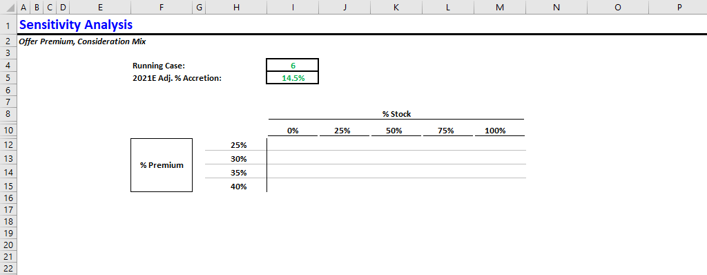
NOTE: we like to include the financial item being sensitized, so that the data table cell formulas don’t have to reference another tab, but that’s just personal preference.
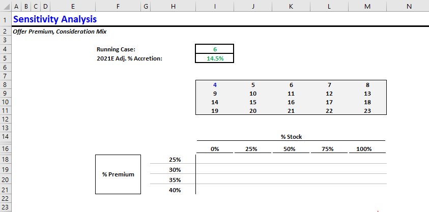
- Next, let’s add the relevant case numbers in a box above the data table. If you’re not sure what I mean, see below. If you go back to the MCASE tab, you will notice that each case (4 - 23) corresponds to one of the data table cells.
- Time to add the actual calculations. Remember the formula:
this cell = if(MCASE = case number, % accretion, this cell)
Try your best to apply the formula, but you can reference the completed sheet if you get stuck.
NOTE: If you get a circular reference warning, you need to enable iterative calculations. Google if you’re not sure what this means.
- If you implemented the formula correctly, only one of the cells in the table should have updated. The rest should be 0. Why? Because we’ve only run one case so far (the current case). Go back to the MCASE tab and run cases 7 and 8. On the Sensitivity tab, you’ll see a couple more cells updated.
As you’re probably thinking, manually running every single case would be super tedious. Fortunately, we have a solution for that. Get ready for some Excel magic.
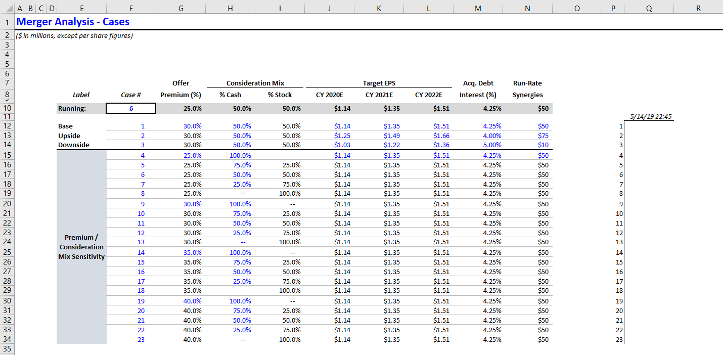
- Go back to the MCASE tab. To the right of your case variables, leave a blank column for spacing and then add two new columns. Set the first column equal to the row’s case number. Leave the second column blank, but at the top (above all case numbers), set a cell equal to the current date.
cell = now()
Here’s what that looks like.
- Now, we’re going to use an Excel data table to run all cases automatically. I know, I know. Data tables are bad, but this is one place where you need them. Typically, my workflow is:
i) Build model
ii) Design outputs
iii) Run cases (via data table)
iv) Delete data table (so model doesn’t lag)
v) Paste outputs
If you need to run the cases again (i.e., to repaste), it’s easy enough to reinsert the data table, and then delete it.
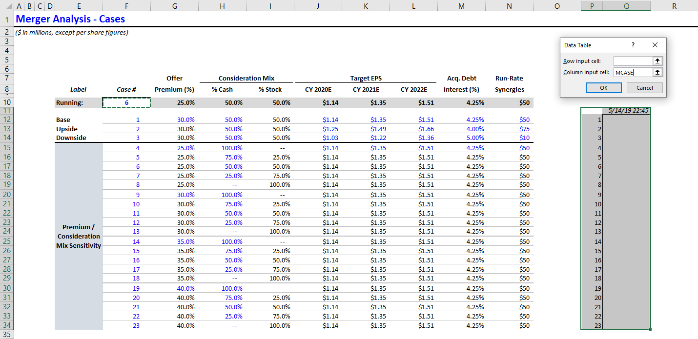
Ok, so let’s add that data table. Highlight the two columns you added (the case column and the empty column with the date on top). Then create a one-variable data table, in which the column variable = MCASE.
Shortcut for data table: ALT + A + W + T
NOTE: you can ignore the row input variable.
Here’s what that looks like.
Press F9 to recalculate the data table. All cases have been run.
Go back to the Sensitivity tab to confirm all cases updated. You should see the following:
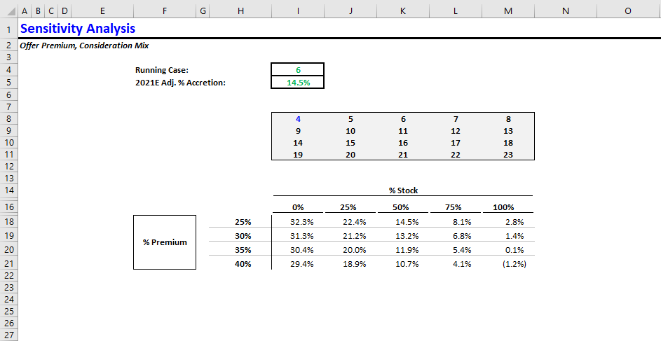
Intuitively, this output makes sense. From the acquiror’s perspective, the most expensive offer package is 100% stock with the highest premium (40%).
Offer Premium & Synergies
Okay, we worked through the offer premium and consideration mix sensitivity analysis together. Try to build a similar sensitivity output for offer premium and synergies. You can use the following synergy values:
- 20mm
- 30mm
- 40mm
- 50mm
- 60mm
We’ll use the same offer premium range. Therefore, we’ll need 25 new cases (5 synergy values x 5 offer premium values). Let’s think about how these 25 new cases will differ from the 25 prior cases.
- Offer Premium: We’re sensitizing offer premium in both, so offer premium values should be the same across both sets of cases.
- Consideration Mix: In the first sensitivity (first 25 cases), we showed varying consideration mixes, whereas in the second sensitivity (next 25 cases), we’ll assume 50-50 cash-stock mix throughout. That’s one difference.
- Synergies Furthermore, in the first sensitivity (first 25 cases), we assumed 50mm run-rate synergies, whereas in the second sensitivity, we’re including a range of synergy values (20 - 60mm). That’s the second difference.
Using this information, try to set up the second sensitivity analysis. If you’re stuck, you can always consult the completed version.
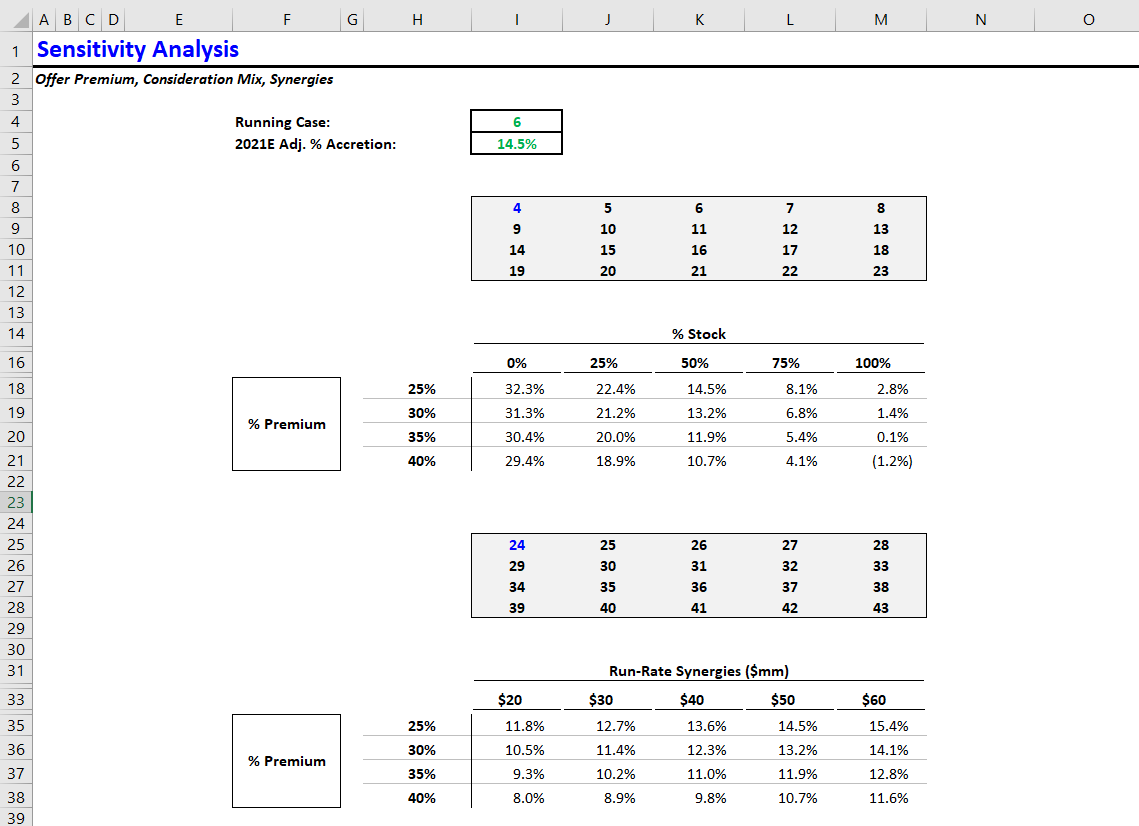
Your updated sensitivity tab (containing both sensitivity tables) should look like this:
Checking Your Work
Bonus points - let’s check those two sensitivity outputs like a VP, who’s not too deep in the weeds.
First, should any of the columns or rows be the same across both tables? (This is called ticking and tying - making sure numbers are consistent across outputs.)
Yes! The first table assumes 50mm run-rate synergies, and the second table assumes 50-50 cash-stock mix. Therefore, the third column (50-50 mix) in the first table should equal the fourth column (50mm synergies) in the second table. We can see that’s the case. So far, so good.
Next, let’s examine each table and verify that the numbers are directionally correct.
We can start with the first table. We know that accretion should decrease when the offer premium is higher (of course, the buyer gets a lower return when they pay more). Therefore, accretion should decrease as we move further down each column. Also, in most cases paying with stock is less accretive than paying with cash. So the leftmost column (0% stock) should have the highest accretion values, and they should decrease as we move right across the table. This checks out.
Now, let’s look at the second table. The same observation regarding offer premium holds: Accretion should decrease as we move further down each column. But unlike the first table, the highest accretion values should be on the right-hand side, because synergies boost accretion. This also checks out.
Conclusion
Now you know the proper way to perform sensitivity analysis. This method is not just for accretion / dilution - it’s for everything. For example, using this approach, you could calculate a sponsor’s IRR under various growth and financing scenarios. It might be intimidating at first, but switching from data tables to self-referencing if statements (+ cases) will speed up your workflow and reduce errors.