Intro
This article is a continuation of our private equity modeling series. We’re going to show you how to take our intermediate LBO template and turn it into a more advanced, flexible LBO model.
There’s a lot of material to cover, so we’re going to split this tutorial into a series of posts. This one will show you how to integrate casing, flexible financing assumptions, and sensitivity analysis. Future posts will cover topics including operating models and add-on acquisitions.
We highly recommend completing the following tutorials before proceeding with this one:
- Intermediate LBO Modeling
- Ability-to-pay Analysis
- Value Creation Analysis
- LBO Equity Waterfall
- Adding Flexible Cases to a Financial Model
- Excel Data Tables, the Right Way
Goal
By the end of this tutorial, you’ll know how to build a sophisticated, flexible LBO model.
Starting Point
As a starting point, we’ll use the completed LBO model from our LBO equity waterfall tutorial.
Download the template, and let’s take a look.
You’ll notice the model includes the following four tabs:
- ATP - this is our ability-to-pay analysis
- Contrib - this is our basic value creation analysis
- LBO - this is our intermediate LBO model
- Equity Waterfall - this is an illustrative equity waterfall
Of these, we’re going to focus almost entirely on the LBO tab. The other three tabs are supplemental analyses, but we’re including them here for the reasons listed below:
- ATP - I include an ability-to-pay analysis with any LBO model. The ability-to-pay analysis is easy to add, and it’s a great sanity check for the LBO.
- Contrib - Likewise, I always include a value creation bridge. It’s important to understand what’s driving the modeled returns.
- Equity Waterfall - This is not relevant in banking, but will be present in any serious private equity deal.
Let’s get started.
1. Financing Cases
In this first step, we’re going to add flexible financing cases to our model. Right now, the financing assumptions are hard-coded at the top of the LBO tab.
First, some general cleanup:
- Let’s move the LBO tab to the far left (out of the four tabs).
- Likewise, since we’ll be adding more tabs to the model, let’s color code the tabs. Make the LBO tab dark blue, and you can make the other tabs all another color.
Now, for the main course.
Create a new tab called FINCASE.
Shortcut for creating a new tab:
Shift F11
Shortcut for renaming a tab:ALT + H + O + RNow, let’s go to the LBO tab and copy the entire financing assumptions table (located at the top of the tab). We’re copying it so that the sensitized assumptions match the LBO format perfectly.
Paste the copied table at the top of the new FINCASE tab starting at cell
I11. The copied table should take up 10 rows, including the blue header bar and the revolver commitment fee.Skip two rows and paste the table again (in line with the table above). Do this two more times. You should now have four copies of the table, with two rows of spacing after each table. The first copied table will be our output, and the remaining three tables will be our financing cases.
We’ll ignore the first table (the output) for now.
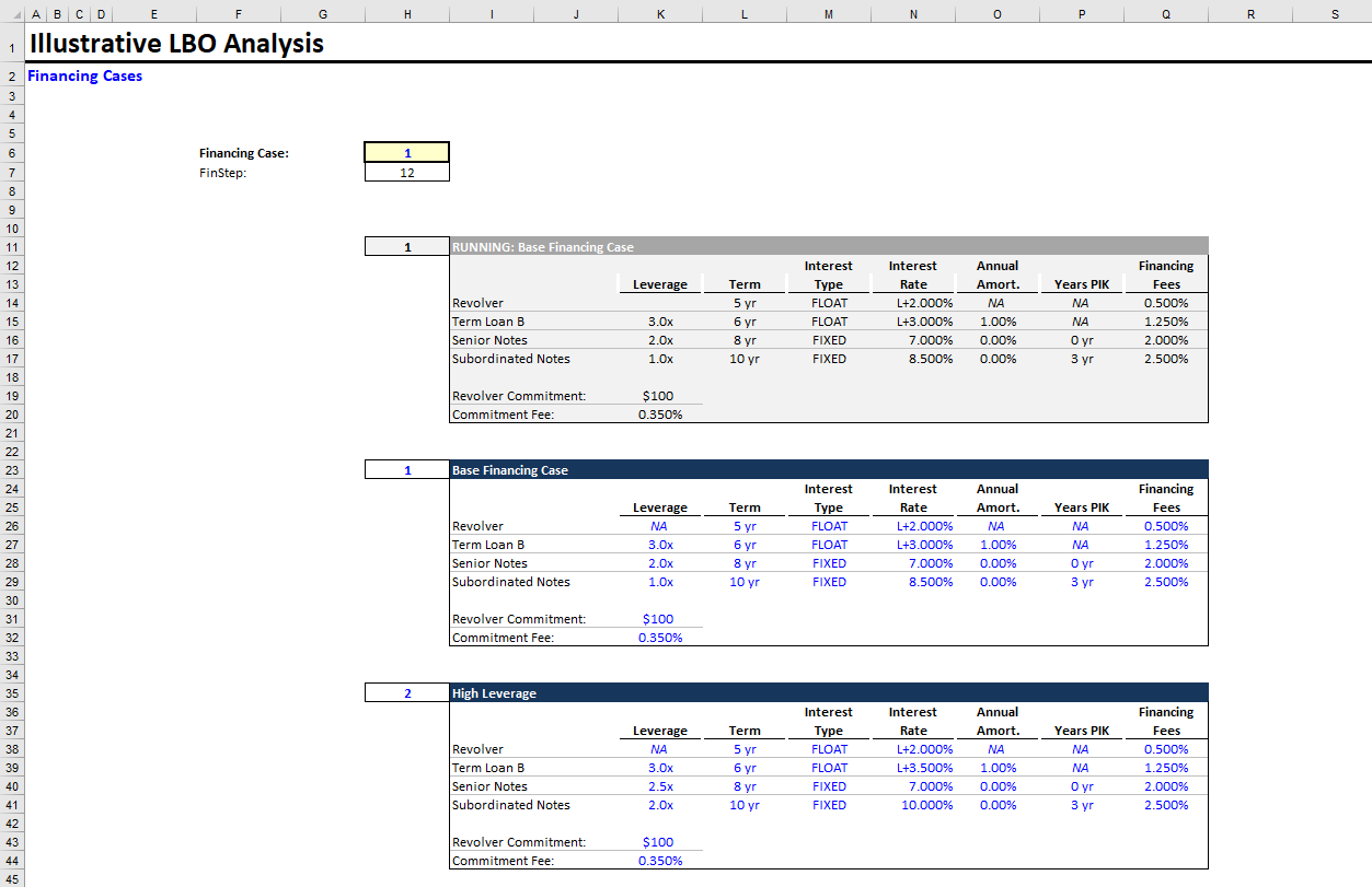
Let’s create our Base Financing Case in the second table. First, change the blue header bar to read
Base Financing Case. Also, let’s reduce the Senior Notes to 2.0x Leverage (giving us 6.0x total leverage).We’ll create our High Leverage case in the third table. Let’s increase the Subordinated Notes to 2.0x Leverage (giving us 7.5x total leverage). Likewise, let’s set the Term Loan B interest rate at
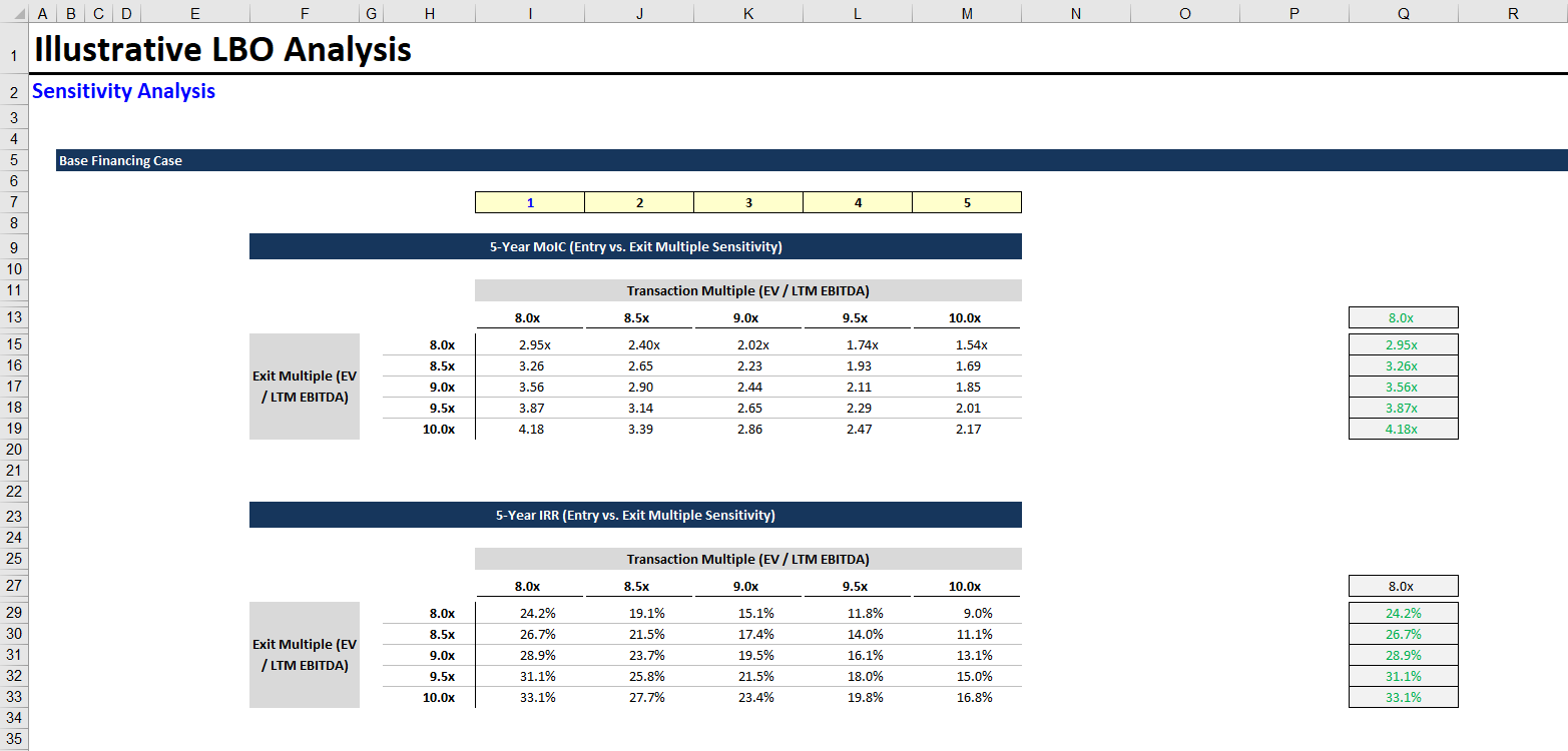
L+3.500%, and let’s increase the interest rate for the Subordinates Notes to10.000%.In the final table, let’s add our Low Leverage case. We’ll set the Senior Notes to 1.5x leverage, and we’ll set the Subordinated Notes to 0.0x leverage (no Subordinated Notes). We can also decrease the interest rates, since we have less leverage (
L+2.750%for the Term Loan B and6.000%for the Senior Notes).Financing Assumptions
Remember: These are illustrative assumptions. You should rely on your capital markets team for up-to-date financing assumptions.Finally, in cell
H6on the FINCASE tab, create a case cell (a thick-bordered cell with a hard-coded number). This is the FinCase cell, which determines the running financing case. You’ll see how it’s used shortly.Directly below the FinCase cell, calculate the total row height of each financing table (we call this the FinStep).
FinStep
Make the formula for cellH7= ROW(High Leverage Header) - ROW(Base Financing Case Header).The Excel ROW function returns the row number for a given cell, so here we’re calculating the total number of rows (including spacing) required for each table.
Formatting: Let’s return to the first financing table (which we referred to as our output). Go ahead and shade the entire table light gray (background color), and make the header bar dark gray. Likewise, change the table font color to black to signify a calculated value (instead of a hard-coded assumption).
Go to the first numerical cell in the output table (revolver leverage - it should read
NA), and use the following formula:= OFFSET(this cell, H6 * H7, 0, 1, 1)
(in English)
= OFFSET(this cell, FinCase x FinStep, 0, 1, 1)FinCase tells us which financing case should be running, and FinStep tells us the required number of rows per table.
Offset Function
If you’re not confident in your understanding of the OFFSET function, please pause this tutorial and Google it. It’s worth 5 minutes of your time. It might be the most powerful Excel function.
We calculated the FinStep (instead of hard-coding it) using the ROW function, so that if we change the number of rows in our financing assumptions, these functions auto-adjust.
Copy this offset formula (but locking the FinCase and FinStep cells) and apply it to all cells in the output financing assumptions table.
Now when you change the FinCase cell (e.g., set the value to 2), the output table should update auto-magically.
Here’s what your completed FINCASE tab should look like:
Last Step
Return to the LBO tab, and link the Financing Assumptions table to the output table at the top of the FINCASE tab. (Remember to change the font color to green to represent a value linked from another tab.) Now when you change the financing case on the FINCASE tab, it updates the LBO tab as well.
Take a second and think about how powerful this is. You can now add as many financing cases as your hyperactive MD could ever desire, and you can update which case is flowing through your LBO model by changing one cell.
Here’s the completed Excel file for this step. Take a look if you’re stuck or want to verify your work.
2. Master Case Tab
In the prior step, we added casing to our financing assumptions. This made our LBO model much more flexible, but that’s not the end of this story.
There are several other variables we want to sensitize that are independent of our financing assumptions (for example, the transaction multiple). How can we sensitive these other variables along with our financing assumptions?
Here, we rely on the concept of a Master Case tab, which is exactly what it sounds like. It’s a tab that rules all the other case tabs and specifies what the running assumptions are. You may be wondering: Why bother putting the financing assumptions in their own tab? And the answer is: Because we generally think about financing assumptions as a single unit:
Analyst: “Yes, this output is based on our conservative financing case.”
VP: “Well, run the aggressive financing case instead and reprint.”
Similarly, we would separate operating model variables into an Operating Cases tab, also controlled by the Master Case tab.
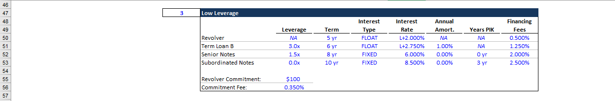
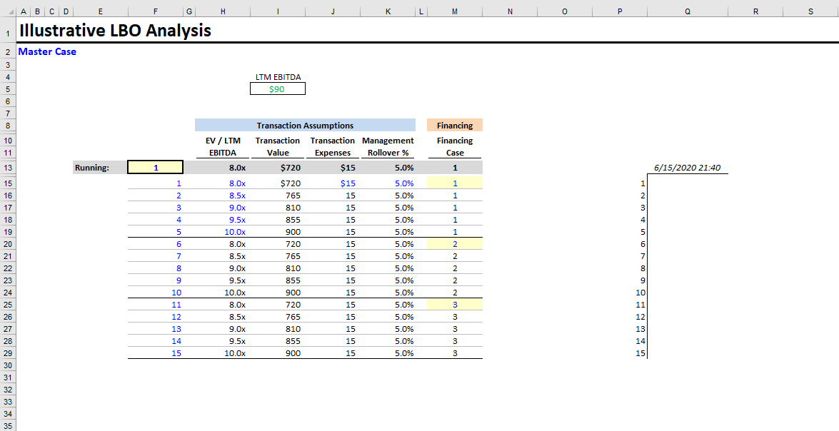
Below is what our completed Master Case tab will look like:
Now let’s build it. Note: This section draws heavily on our Adding Flexible Cases to a Financial Model tutorial, so give that another read if you’re confused.
Create a new tab (named MCASE).
Let’s list the variables we want to include:
- Transaction Multiple (EV / LTM EBITDA) and Transaction Value
- Transaction Expenses
- Management Rollover %
- Financing Case (which financing case is running)
Exit Multiple
We don’t need to include the exit multiple here, because the LBO tab already sensitizes the exit multiple.
- Let’s add the columns. There should be 1 column for each of the variables listed above. I also like to number each case, so the columns should be:
- Case Number (e.g., 1, 2, 3, 4, etc.)
- EV / LTM EBITDA
- Transaction Value
- Transaction Expenses
- Management Rollover %
- Financing Case
Why include both the Transaction Multiple and Transaction Value?
An astute reader might wonder why we’re including both the Transaction Multiple and the Transaction Value in our MCASE tab. After all, doesn’t one determine the other?Yes, that is true. But we include both, because you want to be able to frame the question either way. For example, you might ask “What does a 925mm deal look like?” or “How do the returns look assuming a 10x transaction multiple?” Sure, you could back out the transaction multiple to get to 925mm, but
10.278xlooks rather nonsensical. It will make more sense to someone else, looking at your model, to see 925mm hardcoded directly on the cases tab.
Now, let’s make our first five cases. Across these cases, only the transaction multiple (and therefore, transaction value) will vary; we’ll hold everything else constant. Let’s start the multiple at 8.0x and increase it by 0.5x with each case, so the transaction multiple will range from 8.0x - 10.0x. For the other variables, we can use the existing values hard-coded on the LBO tab (
15mmfor transaction expenses and5.0%for the management rollover). We’ll also set the financing case equal to 1 (our base case). Since only the transaction multiples / transaction values differ, we can hard-code these other variables in the first case (blue font for hard-coded values) and we can set the other rows equal to the preceding row (black font for formulas).Let’s create the Running Case row. Shade the row directly above your new cases medium gray. Likewise, make the font bold and black (for calculated values). In the column where you list case numbers, format the running row cell as a case cell (thick borders, different shading, and blue font).
Name this cell MCASE.
Naming Excel Cells
You can name Excel cells following the steps below:CNTL + F3
New
Enter Name and Press “OK”
When you name a cell, you can reference that cell using its name in other formulas. For example, we’ll be able to refer to the MCASE cell using its name (e.g.,
if(MCASE = 1, ...).Warning
Many analysts have a tendency to go overboard with Excel naming. It is best practice to limit the number of named cells in your model.We want the values in the Running Case row to equal the specified case (the case number in the MCASE cell). Can you figure out how to do this using the
OFFSETfunction? This should feel familiar after the FINCASE tab.Answer
Each cell in the Running Case row = OFFSET(the given cell, MCASE, 0, 1, 1). This just grabs the value from the specified case.Now create the remaining ten cases shown in the picture of our completed MCASE tab (above). You’ll notice that cases 6 - 10 match the first five cases, except for the specified Financing Case, and that cases 11 - 15 also follow this pattern.
Now your MCASE tab is essentially complete. Make any formatting changes in order to match the image above.
Remember: Financial models are, in part, communication tools. They’re a way to examine specific scenarios and share your work with others. Clean formatting is a key part of that.
Here’s the completed Excel file for this step.
3. Connect the LBO & MCASE Tabs
This step is quick. We’re going to connect the MCASE tab with the rest of the model. Once it’s connected, by changing the running case number on the MCASE tab, we update our entire model.
Here are the variables we need to link:
- Transaction Multiple
- Transaction Expenses
- Management Rollover %
- Financing Case
Note: We’re intentionally excluding the transaction value, because it’s already calculated on the LBO tab. I know, I know. We made a big deal about including both the transaction value and the transaction multiple on the MCASE tab, and now we’re only linking one of the values? We included both on the MCASE tab, because we want our cases to be easy to understand. But we only need to link the transaction multiple, because we already calculate the transaction value on the LBO tab. Make sense?
First, let’s link the transaction multiple, transaction expenses, and management rollover percentage on the LBO tab. These assumptions are all hard-coded at the top of the model. Simply replace the hard-coded values with links to the correct cells in the MCASE running row. Remember to change the font colors to green (green signifies a value linked from a different tab).
Last, let’s link up the financing case. Go to the FINCASE tab and set the Financing Case cell equal to the running financing case on the MCASE tab. The Master case tab rules all other casing. It provides a single control panel for your entire model.
Here’s the fully linked Excel file if you want to check your work.
4. LBO Cleanup
This is another quickie. We’re going to make a couple minor changes to the LBO to prepare for the next step.
- Right now, the exit multiples in the LBO returns calculations vary based on the running transaction multiple. We don’t want that anymore. Instead, we want a fixed range of exit multiples.
On the LBO tab, go to the Illustrative Returns section at the bottom of the tab. Hard-code the first transaction multiple in the enterprise value calculations; set it to 7.0x. For the multiple below that, set it to the preceding value + 0.5. Copy this formula down for all the remaining multiples. You should now see transaction multiples ranging from 7.0x to 11.0x in increments of 0.5x.
- Next, let’s put boxes around the returns metrics we’ll use for our sensitivity analysis (next step). Highlight cells
N346:N350(MoIC), and add a border. Do the same for cellsN360:N364(IRR). This serves two purposes:
- Outlining the values will ensure we don’t link to the wrong column (been there, done that)
- Makes it easy to spot check our sensitivity tables in the future
Here’s the updated Excel file.
5. Sensitivity Analysis
This section will walk through adding sensitivity analysis to your model. It draws heavily from our Excel Data Tables, the Right Way tutorial, so if you’re stuck, please reread that article. Long story short: For any sophisticated model, Excel data tables aren’t going to cut it. You need to construct your models with proper casing and sensitivity analysis.
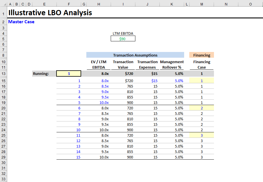
We’re going to make three sets of sensitivity outputs - one for each financing case. Each output will consist of a MoIC (Multiple of Invested Capital) sensitivity table and an IRR sensitivity table. These tables will show our returns metrics at varying entry and exit multiples. Here’s what one of the sensitivity outputs will look like:
Before building the sensitivity output, let’s talk about the various elements in the image above. First, there are the case numbers in the yellow-shaded row. Each column in the output tables is tied to a case number, which refers to a specific case on our MCASE tab. On the right, we see gray-shaded linked values. These are links to the currently running returns metrics on the LBO tab. We also link to the current transaction multiple. Lastly, the values in the sensitivity tables are calculated using the case numbers, these linked values, and the running MCASE.
Enough chitchat. Let’s make some sensitivity outputs.
Create a new tab, and name it Sensitivity.
Add headers and basic formatting to conform to the image above.
Let’s add the case numbers. Each row in the sensitivity tables represents a particular exit multiple (EV / LTM EBITDA). Each column represents an entry multiple (the transaction multiple). We’re fortunate that our LBO tab already sensitizes the exit multiple. Therefore, we can represent each column with a single case (we only need to sensitize the transaction multiple).
The image above shows our entry multiple ranging from 8.0x - 10.0x (same as the exit multiple), which corresponds perfectly to each group of five cases on the MCASE tab. Our first sensitivity output will be for our Base Financing Case, so we’ll use the first five cases (1, 2, 3, 4, 5) here. Fill in the case numbers.
- Next, let’s fill in the gray-shaded linked values. The first cell to link is the transaction multiple. You can set it equal to the running transaction multiple at the top of the LBO tab. Then, the next five linked values are the 5-year MoIC values that we outlined at the bottom on the LBO tab.
For the IRR sensitivity table, we can link the entry multiple to the value above (on the Sensitivity tab). We shouldn’t link to the transaction multiple on the LBO tab again, because we’ve already imported that value. The next five values to link are the 5-year IRR values that we outlined on the LBO tab.
- Last, we’ll create the formulas for our sensitivity tables. We’ll use self-referencing if statements (as described in Excel Data Tables, the Right Way). If you’re not sure what these are, or how they work in the context of sensitivity tables, go back and reread that tutorial. This is a key concept.
You’ll use the following formula for each cell in the data table (including the entry multiple column headers):
= if(MCASE = case number row, linked value column, self)
Make sure to lock the row, for the case number, and the column, for the linked value. This formula ensures that a column only updates when the specified case is running.
You’ll notice that your sensitivity tables have the same values in every column (including the entry multiple column headers). That’s normal! You haven’t run all the cases yet.
- Now we’ll replicate the sensitivity output for our two remaining financing cases.
- First, copy the rows containing both sensitivity tables.
- Then, paste the copied rows beneath the prior output.
- You’ll need to update the case numbers.
- We’ll use the same gray-shaded linked values, but instead of linking to another tab, link to the imported values above. This way, we’re only importing the running MoIC and IRR values once.
- Update self-referencing if statements to use the new case numbers.
You should now have three well-built sensitivity outputs, one for each financing case. Here is the completed Excel sheet if you’d like to compare.
6. Running All Cases
We’ve built our sensitivity outputs. Now we need to run all cases, so that our self-referencing if statements update. To do this, we’re going to use the technique we introduced in our Excel Data Tables, the Right Way tutorial:
- Go to the MCASE tab.
- To the right of your cases, with a couple extra columns for spacing, copy the row numbers. Then, in the running case row above the case numbers, set the cell equal to the current date and time:
cell = NOW()
Your MCASE tab should look like this.
- Next, we’ll use Excel’s native data table functionality to run all cases:
- Highlight the case numbers and date
- Create an Excel data table:
ALT + A + W + T - Enter
MCASEas the column input cell (leave the row input cell blank), and press OK
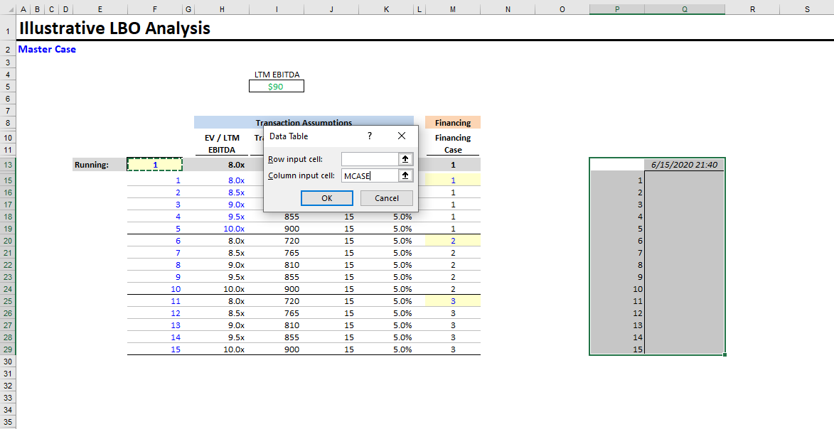
- Press F9 to run all calculations.
- Go to the Sensitivity tab, and confirm that your sensitivity outputs have updated.
Here’s the completed Excel file.
7. Final Cleanup
As a best practice, we don’t like to save Excel files with active data tables. Data tables can really slow down Excel, and self-referencing if statements enable anyone opening the file to see the various scenarios and returns.
Therefore, delete the Excel data table from the MCASE tab and resave the file.
Here’s the final version.
Conclusion
Now you know how to add sophisticated casing and sensitivity analysis to your LBO. Reach out with any questions or feedback.