Introduction

Let’s start with a disclaimer. This article will not serve as an introduction to DCFs and will not cover the WACC calculation. If you have to ask what a DCF is, or how it works, this article is not for you.

This article assumes you have already made at least a couple DCFs and understand the core concepts. This article will walk you through a high-quality DCF template and some of the key considerations.

Some Background

The DCF is the most subjective form of valuation - it is subject to the most judgment and potential for manipulation. When we compare it to other valuation methodologies, it has the most unknown variables.

What are the variables in a DCF?

1. Financial projections
2. WACC (with its own numerous levers and inputs)
3. Exit Multiple / Terminal Growth Rate

The WACC and the Exit Multiple / Terminal Growth Rate are the big unknowns, where investment bankers must exercise judgment. The financial projections are usually supplied by the client, or are created with the client’s input and are subsequently blessed by the client. Investment bankers are not in the business of creating projections, and the client should have a stronger basis to project their own performance.

Compare these unknowns to those of other valuation methodologies:

1. Public trading comparables
2. Acquisition comparables
3. LBO

In public trading comparables and acquisition comparables, there are fewer distinct areas of judgment. The most substantial decision is the first question: which companies or deals are comparable?

Some would argue the LBO is not a valuation methodology, but I’d argue that a LBO performed by a banker is a DCF without the uncertainty of the WACC. The cost of capital for a LBO is mechanical. The illustrative sponsor return threshold is 20 - 25%, and the cost of debt is governed by prevailing debt market conditions - whatever your Leveraged Finance team deems reasonable.

Ok, background aside, let’s check out the template.

Key Assumptions

It’s a best practice to list out your key variables at the top of the file. This allows you to easily keep track of them, and it makes your assumptions explicit to anyone else who might open up the file.

A few notes:

• Perpetuity Growth Rate is just another name for the Terminal Growth Rate.
• Mid-year discounting: This is a boolean switch to turn on mid-year discounting. Mid-year discounting means that for each period of projected cash flows, you assume the cash flows occur in the middle of the projected period, instead of at the end. Otherwise, you’re unfairly penalizing a company’s value if its cash flows occur steadily throughout the year. Here’s an article discussing mid-year convention in depth.

Projected Cash Flows

This section is pretty straightforward. Typically, you would link the financial projections from your standalone projection model instead of hard-coding them here.

One nuance is the “Terminal” year construct. We use this terminal period to normalize the last year of projected free cash flow, and in turn, we use normalized free cash flow to calculate the terminal value via the Perpetuity Growth Method. One common adjustment is to set D&A equal to a certain % of CapEx. Remember, not all CapEx is expensed as D&A. For example, land acquisition costs are not depreciated. All else being equal, a higher % of D&A leads to a higher valuation, because D&A reduces cash taxes paid, thereby increasing cash flow.

Also, the free cash flow is labeled Unlevered Free Cash Flow, because it is unburdened by leverage (debt), i.e., it’s before interest expense. This means these cash flows are the cash flows available to the entire firm, regardless of capital structure. That should tell you that we’re calculating the enterprise value.

You should always ask yourself: Who are these cashflows for? Have any pieces of the capital structure already been paid their due? For example, if we subtracted interest expense and debt amortization, these cash flows would be for equityholders rather than the entire firm.

Terminal Value

As a reminder,

enterprise value = PV of projected cash flows + PV of terminal value

We calculated the PV of projected cash flows in the Projected Cash Flows section of the template. Now we need to calculate the terminal value and then the PV of the terminal value. The two approaches for calculating the terminal value are the Exit Multiple Method and the Perpetuity Growth Method.

It is important to calculate the terminal value using both methods, even if only one of them is appropriate for the valuation (e.g., there are no good comparables, so you can’t find a reasonable exit multiple). Each method acts as a check upon the other.

Perpetuity Growth Method

The perpetuity growth method calculates the terminal value with a perpetuity. How much would this cash flow be worth, grown at X% in perpertuity and discounted at Y%?

The formula (ignoring mid-year discounting) is:

terminal value = terminal free cash flow x (1 + g) / (WACC - g)
PV of terminal value = terminal value / (1 + WACC) ^ 5

But per the discussion of mid-year discounting above, this unfairly penalizes the value of the company - assuming the company’s cash flows occur relatively evenly throughout the year.

The adjusted formula (accounting for mid-year discounting) is:

PV of terminal value = terminal value / (1 + WACC) ^ 4.5

Reasonable Growth Rates
Perpetuity means forever, so you have to be careful with your growth rates. US GDP grows < 3% / year, so a company growing at 5% in perpetuity would eventually overtake the US GDP. Usually, up to 3.00% is standard practice. Here we’re showing 1.00% - 2.50%. You must have a very good reason to go above 3.00%.

Disclaimer: the selection of growth rates and appropriate discount rates can be quite nuanced. The comments above specifically apply to US-based companies and companies in mature economies. It may be appropriate to select higher growth rates for companies based in emerging economies or countries with high inflation, but that is beyond the scope of this article.

Implied Exit Multiple
Using the terminal value (not PV of terminal value), we can calculate the implied exit multiple range. Be consistent with the multiples you’re showing - if you’re using a LTM multiple for the Exit Multiple Method, you should calculate the implied LTM multiple here.

Implied Exit Multiple = Terminal Value / LTM EBITDA

Unfortunately, mid-year discounting makes things more complicated. We assume that the terminal value calculated using the Perpetuity Growth Method (PGM) occurs mid-year, consistent with mid-year cash flow discounting. The Exit Multiple Method (EMM) terminal value, on the other hand, occurs at period end.

To calculate an apples-to-apples implied exit multiple, we need to grow the PGM-derived terminal value by the discount rate for half a period – shifting the value half a period into the future – to make it consistent with the EMM terminal value.

Here’s the revised formula:

Implied Exit Multiple = (PGM Terminal Value x (1 + WACC) ^ 0.5) / LTM EBITDA

A couple notes:

1. The calculation of the implied exit multiple illustrates the intrinsic value relationship between growth and multiples. A higher growth rate leads to a higher value, which leads to a higher implied multiple, and vice versa.
2. If there is a material difference between your implied multiple range and the exit multiple range you’re using, you need to understand why. You may need to adjust your multiple range or your growth rates to achieve consistency.

Exit Multiple Method

The exit multiple method calculates the terminal value by using a multiple at the end of the projection period. You have some flexibility here on which multiple to use. Typically, you use the NTM or LTM EBITDA multiple, but you could also use a revenue multiple. The one constraint is that if you’re performing a DCF analysis on the enterprise value of a company, the multiple should be an enterprise value multiple (so not P/E).

The formula is simple (using LTM EBITDA multiple here):

terminal value = projected LTM EBITDA x exit multiple
PV of terminal value = terminal value / (1 + WACC) ^ 5

Since the terminal value is calculated for period-end, mid-year discounting does not apply to the terminal value. You discount it by the full 5 years.

Check Your Multiple
Selecting an appropriate exit multiple range is key, and it helps to have knowledge of the industry.

1. Is this a cyclical industry? If current multiples are 12.0x, but the historical average is 8.0x, it is NOT appropriate to select 11.0x - 13.0x as your exit multiple range.
2. How are you deriving the exit multiple? Are there good comparables?

Implied Perpetuity Growth Rate
Here is where things get tricky.

We know the formula for terminal value using the Perpetuity Growth Method:

Terminal Value = terminal FCF x (1 + g) / (WACC - g)

We need to factor out the g in order to calculate the implied growth rate. Steps below:

TV = (FCF + FCF x g) / (WACC - g)
TV x WACC - TV x g = FCF + FCF x g
TV x WACC - FCF = (FCF + TV) x g
g = (TV x WACC - FCF) / (FCF + TV)

Ok, not so bad.

But wait. Remember from our discussion of the implied exit multiple that terminal values calculated using the PGM and EMM are inconsistent when we apply mid-year discounting: PGM terminal values occur mid-period, and EMM terminal values occur end-of-period.

We need to adjust the terminal values by half a period of discounting - we are taking the EMM terminal value and discounting it to get the implied PGM terminal value, which can then be used to derive the implied growth rate. The revised formula is as follows:

g = ((TV / (1 + WACC) ^ 0.5) x WACC - FCF) / (FCF + (TV / (1 + WACC) ^ 0.5))

Basically the same as before, but we substitute TV / (1 + WACC) ^ 0.5 wherever we had TV previously.

Check Your Work

If you’re rebuilding this template from scratch, or modifying it, check your work.

One efficient way to check the implied exit multiples and implied growth rates is to plug them into the opposing section. I’ll explain what I mean.

Checking Implied Exit Multiples

1. Copy the row of implied exit multiples (row 65 in the template).
2. Paste the copied values into the row of LTM Exit multiples (row 78 in the template).
3. You should see your assumed perpetuity growth rate range in the implied perpetuity growth rate row (row 82 in the template).
4. Control z to undo the pasted values.

Checking Implied Perpetuity Growth Rates

1. Copy the row of implied perpetuity growth rates (row 82 in the template).
2. Paste the copied values into the Perpetuiy Growth Rate row (row 59 in the template).
3. You should see your assumed exit multiple range in the implied exit multiple row (row 65 in the template).
4. Control z to undo the pasted values.

If your implied values do not match your assumed values when you perform these checks, there is an error.

Example Outputs

The outputs are actually there! They’re just shifted to the right to avoid messing up the column widths of the other sections.

These are the types of outputs I would show for DCFs - a simple presentation of the build to enterprise value.

Introduction

Private equity recruiting has become an earlier and earlier part of the investment banking analyst experience. While all parties acknowledge it’s silly to recruit recent college graduates one to two years in advance, the larger firms don’t want to let their rivals siphon up all the talent, and a prisoner’s dilemma domino effect ensues.

When I recruited for private equity, the main cycle occurred several weeks before most headhunters (claimed they) thought it would (mid-February), and it’s been moving earlier every year.

The early recruiting frenzy has several effects:

1. Academic history matters more than it should.
2. Unequal early staffings can skew recruiting results (over two years this normalizes, but your first couple projects may be the bulk of your pre-recruiting experience).
3. If you want to recruit in the main cycle, you have to make up your mind and prepare early. No time to stop and smell the roses.

These are the unfortunate facts of private equity recruiting. This article will provide some tips and best practices - passed down from older analysts, and learned the hard way.

Rough Timeline

September - November

1. Prepare first version of resume for headhunters.
2. Begin refining “my story.”
3. Schedule headhunter meetings.

October - December

1. Headhunter meetings.

November - January

1. PE firm info sessions / dinners.
2. A few small firms may try to jump the main process and have smaller rounds of interviews.
3. Practice for modeling tests.

January - February:

1. Main recruiting cyle.

Banking + Recruiting?

Banking is a demanding job - tough enough to manage without the stresses of PE recruiting. But the main recruiting cycle is a sprint, not a marathon. You’ll get through it.

Generally speaking, many banks / groups have accepted PE recruiting as a fact of life and try to support their analysts. If you were a summer intern in your current group, you are probably aware of your group’s attitude toward PE recruiting: Do they support it? Is it an open secret? Do the associates or second-year analysts cover for the first-years?

Either way, for your first few months it is best to focus on on the job at hand: being a good analyst. But it is important to get to know the older analysts:

1. They’re generally good people.
2. They can help you acclimate to the analyst role; they can tell you who to work for and who to try to avoid, etc.
3. They probably went through recruiting the year before. They know some of the headhunters and how to prepare.

Tips

1. It is crucial to make a good impression within your group. Headhunters will call older analysts, associates and VPs and make them force-rank the current crop of analysts.
2. Many senior bankers have their own relationships with funds, and can reach out on your behalf. Likewise, some funds will call banks directly in order to diligence analysts further along in the recruiting process.
3. Getting good early staffings can have an outsized impact on your recruiting outcome.

Headhunters

Always keep headhunters’ incentives in mind: headhunters get paid when they successfully place candidates with their client funds (they get paid a lot).

When they meet with you, headhunters are assessing and grading you to determine which client funds they would recommend having you interview with, etc.

First Principles

1. Headhunter meetings are your first interviews. Do not be fooled otherwise.
2. Headhunters are not your friends - they want to place you so they get paid.

Tips

1. Have your story and resume ready before meeting with headhunters. These are your first interviews.
2. Many headhunters have finance backgrounds and can suss out bullshit instantly. Do not exagerate your deal experience. Do not try to “trick” them.
3. There are many headhunters, each representing an array of PE and hedge funds. Your first headhunter meeting probably won’t be your best showing. Schedule the ones you care about least, first. Always good to have a few practice runs under your belt before it counts.
4. If you have genuine, specific interest in one (or a couple) of the headhunter’s clients, tell them. It will show you did your homework, and headhunters know that well-researched, genuine interest translates well with their investor clients (i.e., you have a higher probability to secure an offer + a higher probability you accept = higher probability they get paid from you).

Interviewing

Generally, private equity interviews follow this pattern:

1. Early interviews (with more junior folks)
2. Model test / case study
3. More junior - mid-level interviews
4. Senior interviews
5. Exploding offer?

Interviews test the following skills:

1. Basic financial modeling
   • Model test
   • Paper LBOs
2. “Thinking like an investor”
   • “What’s a good business?”
   • “What makes a good LBO investment?”
   • “What are your main diligence areas for this business?”
3. Personableness / “soft skills”
   • “Tell me about yourself.”
   • “Why PE?”
   • “Why [XYZ] fund / [XYZ] investing style?”

First Principles

1. The modeling test is a way to eliminate candidates. It is a “check-the-box” test – can they do the simple math that is a requirement of this job?
2. Being personable and having a compelling story can smooth over a couple missed investing trivia questions.

Modeling Test Tips

1. Although the modeling test is a check-the-box test, when the main recruiting cycle kicks off, you won’t have time to cram. Preparing early and often is key.
2. Ask older analysts for templates they used to prepare. Study those templates and then build your own.
3. Many PE firms are lazy and recycle the same modeling test every year! If your group has a copy of their old tests, chances are it’s the same one they’ll be using this year.

I prepared by building a new LBO (from scratch) for a different public company every week (November - January). It sucks to spend 2 hours of every Sunday doing that, but in February the preparation is worth it. Make up the projections and some semi-reasonable financing assumptions – the important part is to master the LBO mechanics.

Our LBO model is a great basic template: Training LBO. If you can rebuild this in 2 hours, you will be prepared for any modeling test.

Interviewing Tips

1. You know you will get the following 3 questions every time: (1) Tell me about yourself; (2) why PE / investing; (3) why [xyz] fund / investing style. Master these.
2. Be humble. Your interviewers know you’re essentially a college graduate who’s been sitting in a bank for several months. Express interest and curiosity, but don’t overstate your experience.
3. If you have to choose between preparing for “soft questions” (e.g., tell me about yourself) and practicing “investment” questions (e.g., how to do bond math), choose the soft questions. They’ll come up every time, and you never know what random investment trivia will be thrown your way. (I’ve seen two many smart analysts fail in interviews, because they spent all their time preparing for investment trivia, and not enough time preparing their “soft” pitches.)

Specific Interview Questions

“Tell me about yourself” / “Your story”

• Practice this relentlessly. Having a compelling story is probably the most important factor in your success that you can control.
• 60 - 90 seconds (max). No one wants to listen to you drone on and on. They will ask you questions if they want to hear more about something.
• This is a narrative, and NOT a recitation of achievement. They have your resume. This is the personal narrative that connects the resume dots, and helps you stand out in their minds when they’re comparing candidates later.
• Things to include: (i) where you grew up, (ii) why you went to your college, (iii) what you studied in college and why, (iv) how that led you to banking, (v) any other fun facts (e.g., I grew up on a working farm and could drive a tractor before I was 10)
• Your story should help them understand your journey, and it should end leading into why you’re interested in PE.

“Why investing / private equity”

• “Because I want to make a lot of money” is not a good enough answer.
• Ideally ~30 - 45 seconds
• Have you always been interested in investing? Do you have talking points backing that up (e.g., investing in public markets since I was 10)? If you haven’t always been an investing nerd (that’s ok), what sparked your curiosity? How has banking made you more interested in the investing world?
• You should touch on why PE vs. other forms of investing - you don’t want them to think: “Ok, he / she loves trading stocks and will just leave for a hedge fund in a couple years.”

“Why [xyz] investing style / fund”

• This ties into the answer above.
• For each fund you interview with, you should look up their prior deals and have specific questions. You should understand their investment style and what types of assets they like.
• This is especially important for non-vanilla funds / strategies (growth equity, distressed investing, specific industry focus, etc.). They know they’re not quite like everyone else, and they want to know why you like that.

Choosing a Fund

For many analysts, the prevailing attitude is: take the most prestigious option you can get. If you have multiple options, you should think carefully about your long-term goals and how the various funds fit with those goals.

Some questions you should think about:

1. Do you want to go to business school?
   • Which schools do a fund’s associates typically attend?
   • Where did the partners go to business school? (You hope they’ll write your recommendations)
2. Do you want to avoid business school?
   • Does the firm promote internally without business school? Is this semi-regular or a rare occurrence?
3. Are you passionate about a particular industry?
   • Can you be guaranteed placement in that vertical / team?
   • Do they have a strong investment track record in that industry?
4. How has the firm performed (historically and in the latest fund)?
   • Are they going to be able to raise another fund (so that you’re not just performing portfolio maintenance)?

Diligencing PE Firms

They interview you, but you are also interviewing them. Unfortunately, given the short time-span of the main PE recruiting cycle, even if you have multiple options, it can be difficult to make an informed decision.

Some things to look for:

1. How involved in the recruiting process are the current PE associates? Do they run the process, or do you never even meet them? This can be a good indication of how much responsibility they’re given and what the team dynamic is like. (I saw both extremes and everything in between.)

2. If the firm sends PE associates to business school and recruits post-MBA associates / VPs, do the pre-MBA associates come back after school? If not, this points to some combination of the following:

   • The PE firm is bad at picking associates who make good long-term team members.
   • The pre-MBA experience is so bad, they don’t want to come back.

3. Are the men wearing ties / what is the dress code? This probably gives some indication on how laid back (or strict) the culture is.

4. What types of questions do they focus on? Do they care about getting to know you, or do they focus on solely your knowledge of financial trivia?

These are just some examples. If you pay attention while touring various firms and interviewing, you can pick up clues that may help inform your decision. Speak with older analysts in your group, too.

Good luck.

1. Introduction

Which factors are driving most of the sponsor returns?

It can be tricky disentangling the different value drivers contributing to your rosy 25% IRR. It’s important to do so, however, for many reasons:

• Is debt paydown or EBITDA growth contributing most of the returns?
• Are these growth assumptions defensible?
• Uh oh, we’re assuming 90% of the value creation comes from debt paydown and multiple expansion…

You get the idea.

This can be useful on both the buyside (before presenting your model to a superior) and the sellside (making sure that sellside case is somewhat defensible).

This tutorial is going to build off the prior two articles, and you’ll learn how to put together a value creation bridge - showing where the sponsor returns are really coming from.

Here is what the completed analysis looks like:

You can reference the completed excel file.

2. Fundamentals

Sponsors grow the equity value of their investments using two levers:

1. Increasing the Total Enterprise Value (TEV)
2. Debt Paydown - thereby increasing the portion of Total Enterprise Value allocated to equityholders.

Value creation from the sponsor’s perspective is:

Value Creation = Exit Equity Value - Equity Invested

This can be expanded to separate the impact of debt paydown from the change in Enterprise Value. These are the two levers from above:

Value Creation = Change in Enterprise Value + Debt Paydown

While debt paydown is simple to measure (that’s what the LBO model tracks), the change in enterprise value can be separated into different variables.

3. Decomposing Change in Enterprise Value

Enterprise Value, otherwise known as Transaction Value, is usually calculated:

Transaction Value = Adj. EBITDA x Transaction Multiple

Therefore, the change can be separated into these two buckets:

1. Change in multiple (a.k.a. Multiple Expansion) and
2. Change in EBITDA.

Change in EBITDA can be further decomposed into revenue growth and margin enhancement. For example, cost savings might not contribute any revenue growth, but would increase the EBITDA margin. We’re keeping the change in EBITDA in a single bucket here though, because in our dummy operating case we keep margins constant. Therefore, all of the EBITDA growth comes from revenue growth.

4. Takeaways

In our illustrative output above, you can see that ~50% of total value creation comes from EBITDA growth, and since margins are constant, we assume revenue is the primary driver.

On the buyside, it would be important to diligence the specific assumptions underlying that revenue growth. Especially for a larger company, you would probably have a detailed operating build for each of the different business segments. Maybe one segment in particular is driving most of the growth.

On the sellside, you know that sponsors will do this analysis, and they will focus on the key diligence points. You can help management prepare for the areas that will receive the most attention.

5. FAQ

Why are you adding fees to calculate the initial sponsor equity?

Because we’re calculating how much money the sponsor needs to invest, and they need to pay for fees. Therefore, bigger fees require a greater sponsor investment.

Why are you subtracting fees from the sponsor exit value?

Again, the sponsor needs to pay for fees. This value creation analysis is net of fees. Any money the sponsor receives comes after paying down debt and transaction fees.

For the entry calculations, why are you using total debt (600mm) vs. net debt (595mm)?

If you were wondering this, congrats - you’re being a careful reader.

The entry column must match the sources & uses. We assume 5mm minimum cash balance, so that cash isn’t available for the transaction. It’s the cash required to run the company and fund working capital. Therefore, we’re treating the 5mm of cash as an operating asset and ignoring it for the purposes of the transaction.

So why are you using net debt to calculate the exit value?

Good job picking up on this inconsistency - you may make an astute MD one day.

The entry column must match the sources & uses. That’s why we’re excluding the minimum cash balance there.

The exit column returns should match the returns included in the LBO. Therefore, we need to use the same net debt figure. In the LBO returns section, we try to keep it simple by calculating net debt as all debt minus all cash.

This leaves us with the aforementioned inconsistency in the treatment of operating cash. It’s important to recognize that this inconsistency stems from how we treat operating cash in the LBO. It is not a new assumption introduced in the value creation analysis.

If you spotted this inconsistency while exploring the value creation analysis, then I would argue that this exercise was successful. It led you to think critically about our assumptions and what really generated the modeled returns.

Hold up, why aren’t you subtracting fees in the LBO returns calculations?

Alright, you caught me. That’s another inconsistency. Generally, for high-level LBOs like this one, you don’t subtract future transaction fees in the returns calculations.

We’re including the fees in the value creation analysis, because it felt inconsistent to include the impact of the fees at entry and not at exit (especially when they’re side-by-side).

If you set the exit fees to 0, the calculated exit equity value and MoIC will match the values calculated in the LBO.

6. Next Steps

Try the rest of our private equity modeling tutorials:

1. Easy LBO
2. Intermediate LBO Guide
3. Advanced LBO Guide
4. Ability-To-Pay Analysis
5. Dividend Recap Guide
6. Private Equity Modeling Guide

1. Introduction

How much can a financial sponsor afford to pay?

This is the question that an ability-to-pay analysis strives to answer. On the sellside, bankers use this analysis to frame sponsor bids. On the buyside, sponsors perform similar sensitivity analyses when determining potential bids. The key assumptions are the operating projections and the financing case.

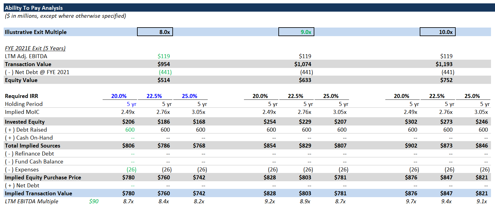
Here is what the completed analysis looks like:

Try to build the ability-to-pay analysis on your own, but you can use this completed version as a reference.

2. Calculate Equity Invested

You should build your ability-to-pay analysis after building your LBO, because many of the key inputs come directly from the LBO.

The key concept to understand is: in an ability-to-pay analysis, you work backwards.

What does that mean?

Well, we know most sponsors have an IRR threshold of 20% - 25%. They won’t be interested in a transaction if they don’t expect to achieve an IRR within that range. Since we’re taking the current operating case as a given, we know the 5-year projected EBITDA, so we can calculate the transaction value at exit. We have the assumed financing case as well, so we know what the cumulative debt paydown and future net debt will be.

Equity Value = Transaction Value - Net Debt

Using the projected EBITDA and a range of exit multiples, calculate the implied transaction value at exit. Then, subtract future net debt (at exit) to derive the future equity proceeds to the sponsors.

Next, using the IRR threshold (20% - 25%), calculate the maximum equity check size. There are a couple ways to do this:

Option 1

Max Equity Invested = Equity Value @ Exit / (1 + IRR) ^ 5

Option 2

Calculate the MoIC as an intermediate step. MoIC = (1 + IRR) ^ 5
Then divide future equity value by MoIC. It’s the same thing, just broken into 2 steps.

Now we have the maximum equity check size, but we need to calculate the implied entry multiple.

3. Calculate Total Sources

To go from maximum equity investment to implied entry multiple, we need to back out the sources and uses. Given our cash-free, debt-free transaction, this is pretty simple, but it can be more complicated.

In addition to the calculated sponsor investment, we have the debt financing assumptions from the LBO. Since we’ve been lumping management rollover and sponsor equity together for returns calculations, we don’t need to add the management rollover amount. It’s implicitly included in the maximum equity investment.

Calculate total sources:

Total Sources = Maximum Equity Investment + Total Debt Raised

4. Implied Transaction Multiple

Next, let’s subtract any refinanced debt (there is none) and expenses. All remaining sources of cash can go towards the equity purchase price. Combining the equity purchase price with net debt, we get the implied transaction value (here, equal to equity purchase price). Divide by 2016A Adj. EBITDA to derive the entry multiple.

Note: we could have subtracted transaction expenses from total sources to calculate the implied transaction value, but we wanted to lay out all of the sources & uses line items.

5. Check Your Work

There’s a neat way to check your work: You can plug the implied transaction multiple back into the LBO as the entry multiple, and the calculated IRR (in the Sponsor Returns section) should exactly match the corresponding IRR threshold.

Example: Use the implied entry multiple assuming a 20% IRR over 5 years and a LTM exit multiple of 9.0x. If you plug that implied entry multiple into the Transaction Assumptions section, the 5-year IRR should be exactly 20.0%.

If yours doesn’t match, double check your model against the provided Excel file.

6. Next Steps

Try the rest of our private equity modeling tutorials:

1. Easy LBO
2. Intermediate LBO Guide
3. Advanced LBO Guide
4. LBO Value Creation
5. Dividend Recap Guide
6. Private Equity Modeling Guide

1. Introduction

This guide will provide basic instruction on modeling LBOs. Specifically, you will learn:

• How to build a full-featured LBO model
• Some key Excel functions
• Core financial concepts and terminology
• How to model different types of debt

This guide will not serve as:

• An introductory accounting course
• A “from-the-ground-up” Excel course

If this model is too complicated, start with our Easy LBO Guide.

LBO Overview

LBO means “Leveraged BuyOut.” Two main characteristics differentiate LBOs from other types of acquisitions:

• Instead of a “corporate” buying another “corporate,” e.g., Amazon buying Whole Foods, in a LBO, a Financial Sponsor (a.k.a. private equity firm) is the buyer
• The sponsor uses a mix of debt (hence “Leveraged”) and equity to buy the company. The equity is the money that the financial sponsor invests, and sponsors raise debt financing from banks / the capital markets.

Do sponsors buy the whole company?
In LBOs, the sponsor generally buys a controlling stake in the company. Management and/or the seller may retain some equity.

Why does a sponsor use debt?
A sponsor uses debt so that they can buy the company with less of their own cash (equity). Over time, as the company pays down its debt, the equity value will grow as a percentage of the total enterprise value, thereby increasing the value of the sponsor’s investment.

Total enterprise value (TEV) = equity value + net debt.

If enterprise value is increasing and net debt is shrinking, the sponsor is simultaneously using two levers to increase their equity value:

1. growing TEV and
2. increasing the percentage of TEV owned by equityholders.

Debt Primers

If you don’t have a decent understanding of the different types of debt used in LBOs, spend ~15 minutes perusing the guides below. A quick read will give you the background knowledge you need.

• LeveragedLoan.com
• S&P Guide - Leveraged Loans
• HighYieldBond.com
• S&P Guide - High-Yield Bonds

2. Getting Started

Download the following files:

• Blank Model - you’ll build your own model with this template.
• Completed Model - for your reference. This Excel file includes a tab for each step of the tutorial. Note: the numbering starts at 3; the first step is the tab labeled “LBO_3” - “3. Filling in Transaction Assumptions.”

You should try to follow along, step-by-step, building your own model from the blank file.

Our model template is built vertically within a single tab, and is divided into the following sections:

• Transaction Assumptions
• Income Statement
• Working Capital Schedule
• Balance Sheet
• Statement of Cash Flows
• Debt Schedule
• Interest Expense Schedule
• Credit Metrics
• Returns Calculations

For simpler LBOs, like this one, we prefer a single-tab, vertical format, because it makes it easier to link between sections and trace dependencies.

The working capital schedule and balance sheet are often unnecessary, but we’re including them here so you can see how all the pieces fit together. Likewise, the debt schedule and interest expense calculations are usually bundled together, but since they’re a bit longer here, we split them up.

3. Filling in Transaction Assumptions

At the top of the “LBO” tab, you can find the Transaction Assumptions section. This is where we’re going to start, and there’s a lot going on, so we’ll go through a brief overview:

• The Sources & Uses section is one of the key parts of any financial model. Quite literally, it describes what your sources of cash are, and what you’re using them for. In LBOs, your sources will be a mix of debt and equity financing, and your main use will be purchasing the target company (“Purchase Equity”)
• The Transaction Assumptions section is where we’ll calculate the transaction value / equity value. In an acquisition, “transaction value” is equivalent to “total enterprise value” (TEV). Therefore, equity value = transaction value - net debt. We’re going to assume a cash-free, debt-free transaction, which means the sponsor is buying the company with no debt to refinance and no excess cash (there will be a little bit of operating cash).
• The Financing Assumptions section contains financing assumptions for various tranches of debt (we provide these). We’ll show you how to use these inputs to perform the financing calculations required in a LBO.

Transaction Value & Equity Value

1. Link the LTM Adj. EBITDA from the income statement (use 2016A - we’re assuming an illustrative transaction close at FYE 2016).
2. Calculate the Transaction Value (LTM Adj. EBITDA x Transaction Multiple).
3. Link the “Cash On-Hand” from Sources as the cash balance.
4. Link “Refinance Existing Debt” from Uses as the debt balance.
5. Equity Value = Transaction Value - Debt + Cash
   Hint: transaction value and equity value should be the same in this case (cash-free, debt-free).

Management Rollover
In a management rollover, the management team agrees to “roll over” part of their equity stake as an investment alongside the financial sponsor. A management rollover is not uncommon, and sponsors like it, because it keeps the management team even more incentivized. If check size (how much money a sponsor is able to invest in a single deal) is a concern, a management rollover can help mitigate that.

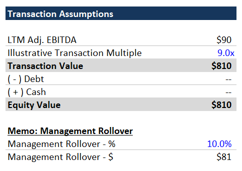
Here we’re assuming a 10% rollover. This means that the management team owns at least 10% of the existing equity and agrees to keep 10% invested alongside the sponsor. 10% is probably a bit high, but not unheard of. Multiply the rollover % by the calculated equity value.

4. Purchase Accounting

We’re using overly simplified purchase accounting, because frankly, purchase accounting isn’t very important for LBOs.

The core concept of purchase accounting is that the value paid for an asset must be capitalized on the balance sheet. In the case of an acquisition, the asset being acquired is the company itself and its bundle of assets and liabilities.

In most acquisitions (including this one), the price paid exceeds the existing book value of net assets. Therefore, the purchase price is allocated to the net assets by writing them up to fair value.

Example: you buy a manufacturing company for $500mm. The net assets have a book value of $100mm, so there’s a $400mm delta, but the fair value of the company’s manufacturing PP&E is actually $200mm. On the balance sheet of the post-acquisition company, the PP&E is written up to $200mm. But that doesn’t cover the full delta - so what next? Any remaining purchase price is allocated to an indefinite-lived intangible asset called goodwill (“indefinite-lived” is just an accounting term that means it doesn’t have a finite life. Theoretically, it could last forever).

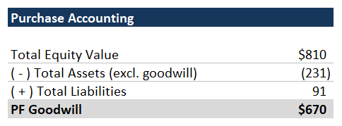
Here we’re assuming that the book value of net assets (excluding the existing goodwill) is equal to fair value, so the entire excess purchase price is allocated to goodwill.

1. Set Total Equity Value equal to the Equity Value you just calculated above.
2. Link the appropriate asset & liability fields from the balance sheet.
   • Remember to subtract out the existing goodwill (goodwill functions as the plug; we don’t care about the prior plug – we’re calculating it again here).

5. Debt Financing

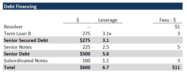
Now we’ll fill out the Debt Financing section below the provided financing assumptions. Here we’ll calculate the actual amount of debt raised and associated fees.

1. For the Revolver, link to the hard-coded “Revolver Draw” assumption under Sources. The assumed draw is $0, which is standard practice. It would be unusual to fund the transaction with the Revolver. The Revolver functions as a safety net, and it is used to fund any short-term cash shortages.
2. Calculate the $ raised for the Term Loan B, Senior Notes and Subordinated Notes using the supplied leverage multiples and LTM Adj. EBITDA.
   • Simply multiplying the leverage multiple by Adj. EBITDA can result in oddly specific debt balances (e.g., $179.4mm of senior notes), whereas companies raise round numbers of debt.
   • Use the mround function and the “Minimum Debt Increment” assumption found under Other Assumptions to get nice, round debt balances for each tranche:

     =mround(leverage * EBITDA, minimum debt increment)

3. Calculate the financing fees for each tranche by multiplying the calculated debt balance by the fee % from the Financing Assumptions table.
   • For the revolver fee, multiply the financing fee % by the revolver commitment.

6. Sources & Uses

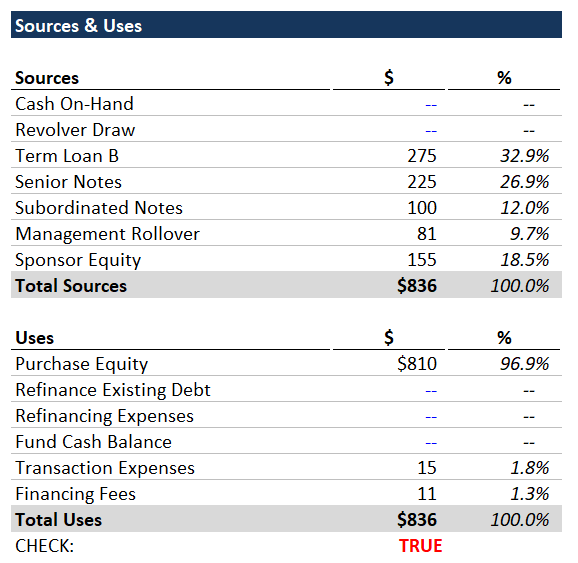
Now we’ll fill out the Sources & Uses using our work from the preceding sections.

1. Under Sources, link the individual debt tranches from the Debt Financing section.
2. Link Management Rollover from Transaction Assumptions.
3. Under Uses, set Purchase Equity equal to Equity Value from Transaction Assumptions.
4. Link Transaction Expenses from Other Assumptions.
5. Link the Total Financing Fees from the Debt Financing section.
6. Now the only remaining line item is Sponsor Equity; set it equal to Total Uses - the sum of all other sources.

   Sponsor Equity = Total Uses - Sum(All other sources)

Your Sources & Uses should now balance.

7. Income Statement

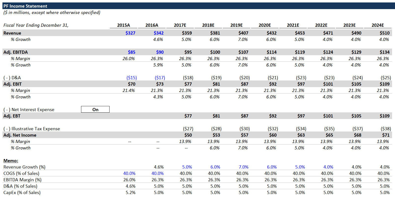
Let’s fill out the PF Income Statement. The historical revenue, EBITDA and D&A are already in place, and we’ve included all the assumptions you need in a memo below the income statement.

1. Grow Revenue by multiplying the prior year by (1 + growth rate).
2. Calculate projected EBITDA by multiplying margin by Revenue.
3. Calculate D&A with the % of sales.
4. Subtract D&A from EBITDA to arrive at EBIT.
5. Leave Net Interest Expense blank for now, but calculate EBT as EBIT + blank Net Interest Expense row.
   • EBT equals EBIT for now, but we will add Net Interest Expense in the future.
6. Calculate tax expense by multiplying the tax rate found in Other Assumptions by EBT.
7. Calculate Net Income by adding the tax expense (negative) and EBT.

8. Working Capital Schedule

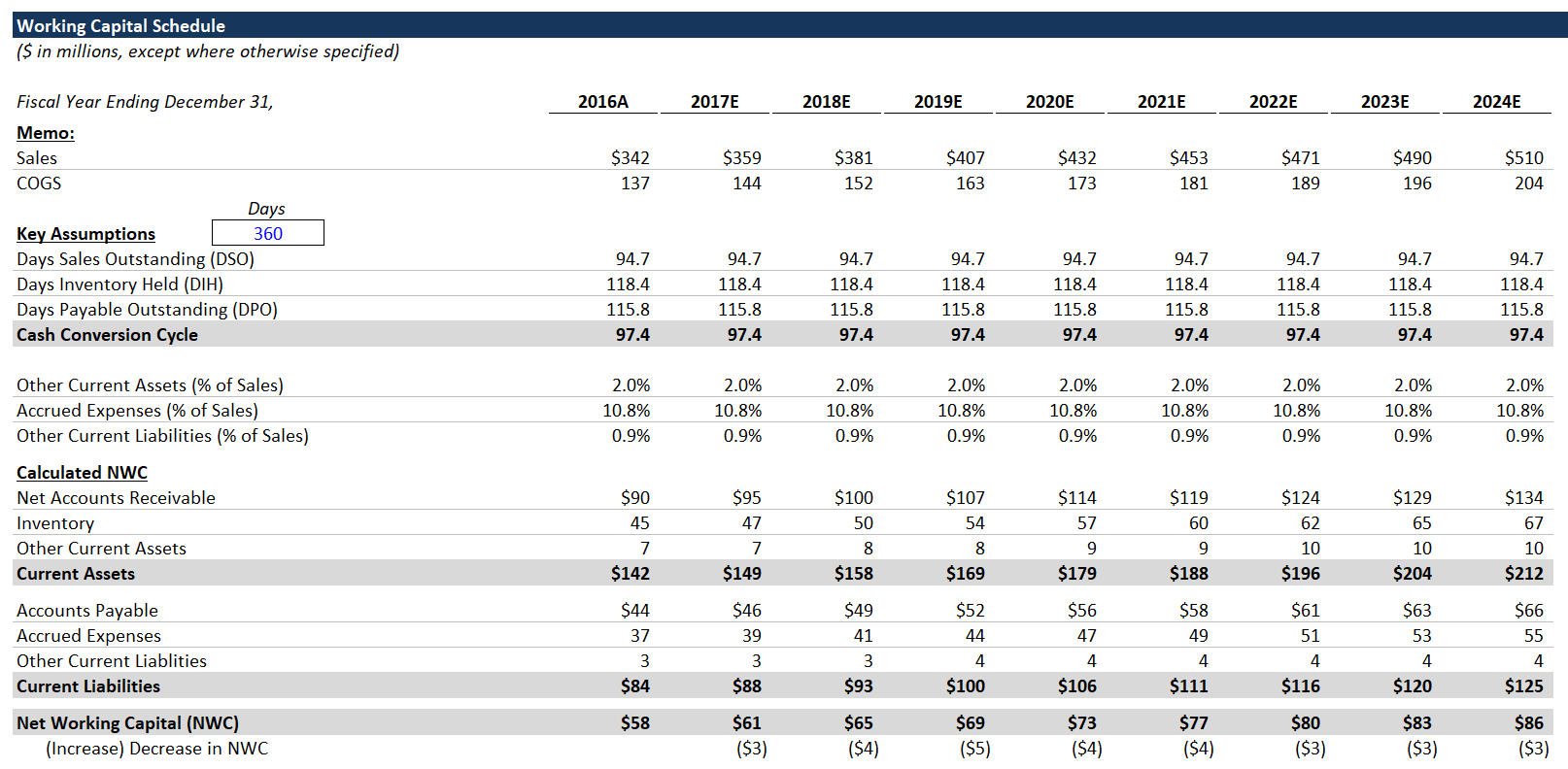
We’re going to use Revenue, COGS and historical working capital to build out the Working Capital Schedule.

1. Set Sales equal to the Revenue line in the Income Statement.
2. Calculate COGS by multiplying Sales by the COGS memo line in the Income Statement.
3. Link the 2016A working capital line items from the Balance Sheet:
   • Net Accounts Receivable
   • Inventory
   • Other Current Assets
   • Accounts Payable
   • Accrued Expenses
   • Other Current Liabilities
     We’ll use these to calculate the historical ratios, which will be the basis for our projections.
4. Calculate the historical DSO, DIH, DPO and % of sales metrics. For metrics based on days, use the provided 360-days cell.
   • DSO = Net Accounts Receivable / Sales * 360 Days
   • DIH = Inventory / COGS * 360 Days
   • DPO = Accounts Payable / COGS * 360 Days

     Cash conversion cycle is a common metric for working capital efficiency. Cash conversion cycle = DIH + DSO - DPO. Time that cash is invested as inventory + time that the accounts receivable are outstanding - the time that the company can delay paying its account payables.

5. Once you’ve calculated the historical ratios for 2016A, set the ratios in all the future years equal to 2016A. This is a simplifying assumption - in a real LBO, it would be important to diligence all these assumptions and have a detailed view on how/why a company’s working capital profile might change.
   • By holding these ratios (and COGS as % of Sales) constant, we’ve made working capital a linear function of Sales.
6. Use the projected working capital ratios (held constant) and the projected Sales & COGS to calculate the projected working capital line items.
   • Example: Projected Inventory = DIH / 360 * COGS
7. Calculate Net Working Capital (Current Assets - Current Liabilities) in each year.
8. Calculate the (Increase) Decrease in NWC as: prior year Net Working Capital - current year Net Working Capital. We do it this way (so that increases are negative), because we’re going to link this line directly to the Statement of Cash Flows. Increases in NWC are a use of cash, and decreases are a source of cash.

9. PF Balance Sheet

We’re assuming that the transaction closes at Fiscal Year End 2016. FYE 2016 has already come and gone, but best practice is to use the latest available balance sheet. For a public company, you’d use the latest 10-K/10-Q.

The historical 2016A balance sheet that we have here is the company’s standalone balance sheet (assuming no transaction). We’re going to calculate the PF 2016 balance sheet - what the balance sheet would look like immediately after closing the transaction.

When preparing a PF balance sheet, incorporate all line items from the Sources & Uses. You can set balance sheet line items that aren’t affected by the Sources & Uses equal to the standalone balance sheet.

1. Set all working capital line items equal to 2016A:
   • Net Accounts Receivable
   • Inventory
   • Other Current Assets
   • Accounts Payable
   • Accrued Expenses
   • Other Current Liabilities
2. Set Net PP&E and Other Noncurrent Liabilities equal to 2016A.
3. The PF Shareholders’ Equity = Sponsor Equity + Management Rollover - Transaction Expenses. You can completely ignore the historical equity balance.
4. Debt = sum(all sources of debt financing).
   • Make sure to include the line for the revolver draw even though it’s 0.
5. Other Noncurrent Assets = 2016A balance + Financing Fees.
   • Financing Fees are capitalized and then amortized over the term of the debt instruments, and best practice is to stick the capitalized fees in Other Noncurrent Assets.
6. Goodwill = PF Goodwill, which you calculated in the Purchase Accounting section.
7. Set Cash & Cash Equivalents = 2016A cash balance - “Cash On-Hand” + “Fund Cash Balance.” Since these latter two are both $0, PF cash = 2016A cash.

Your PF balance sheet should now balance.

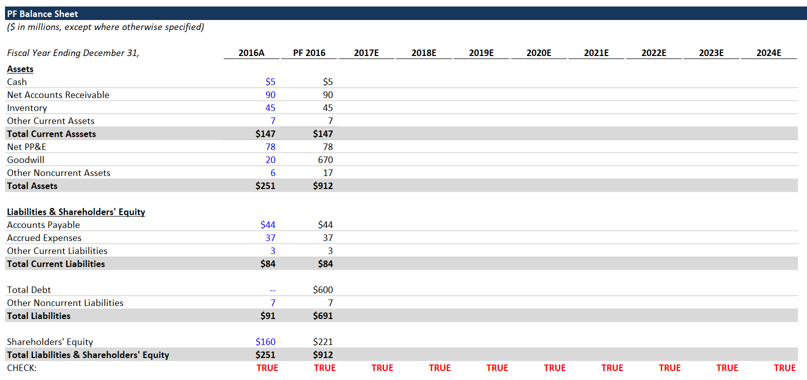
Getting the balance sheet to balance can be tricky. A good way to think about it is that if the historical balance sheet balances and the sources and uses section balances, the combination should also balance. Every line item in sources & uses must be accounted for in the PF balance sheet. The sources are generally straightforward. Goodwill and any purchase accounting write-ups are the bridge between the equity purchase price and historical net assets.

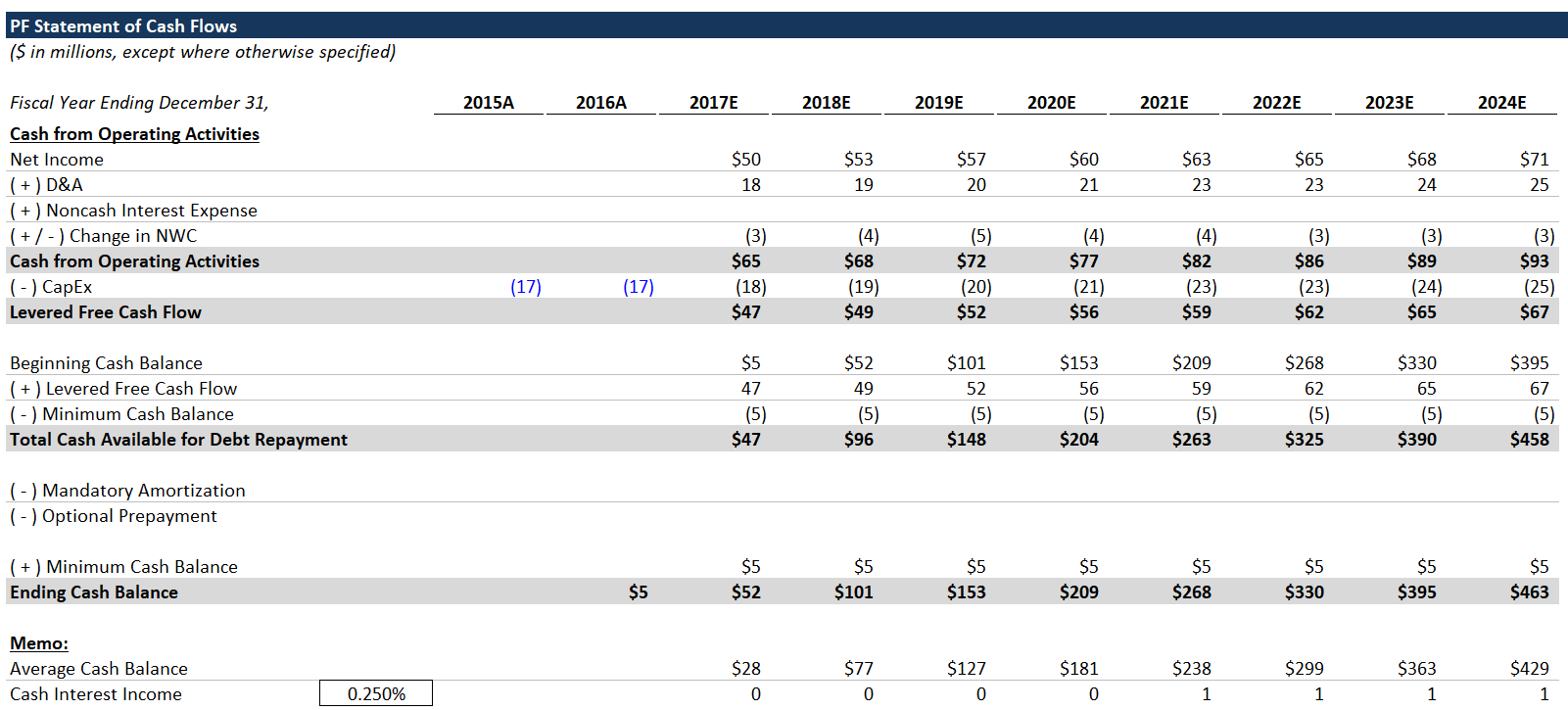
10. Statement of Cash Flows

1. Link Net Income from the income statement. You can ignore the historical years; we only care about the cash flows going forward.
2. Add back D&A (noncash expense).
3. Link to the (Increase) Decrease in NWC from the Working Capital Schedule.
4. Leave Noncash Interest Expense blank for now.
5. Calculate projected CapEx as a % of Revenue (assumption found in the memo section below the Income Statement).
6. Add up the Cash from Operating Activities and Levered Free Cash Flow lines.
7. Link the 2016 Ending Cash Balance from the PF 2016 cash from the balance sheet.
8. Set the 2017E Beginning Cash = to the 2016 Ending Cash (in statement of cash flows).
9. Calculate Cash Available for Debt Repayment:
   • Add Levered Free Cash Flow.
   • Subtract the Minimum Cash Balance (from “Other Assumptions” section).
   • The Minimum Cash Balance ensures that a minimum amount of cash remains - the cash needed for ordinary operations.
10. Leave the Mandatory Amortization and Optional Prepayment lines blank.
11. Add back the Minimum Cash Balance above Ending Cash.
12. Then calculate Ending Cash:

    Ending Cash = sum(Cash Available for Debt Repayment, Mandatory Amortization, Optional Prepayment, Minimum Cash Balance).
    We add back the Minimum Cash Balance, because it was never spent. It was just taken out of Cash Available for Debt Repayment.

13. Carry over these formulas through the rest of the projection period.

Interest Income
Now we’ll calculate Cash Interest Income. Although it’s immaterial, it’s still best practice to include this. We’re going to use an “if” statement to manage circular references.

Average Cash Balance = if (CIRC = 1, average(Beginning Cash, Ending Cash), Beginning Cash)
The circ is found under “Other Assumptions.”

Calculate Cash Interest Income by multiplying the provided interest rate by the Average Cash Balance for each year.

11. Debt Schedule

1. To start, link the PF 2016 ending debt balances from the Sources & Uses. Sum them up in the total line.
2. Calculate the Undrawn Revolver Commitment:

   Undrawn revolver commitment = max(0, revolver commitment - the drawn balance)
   Include “max(0, “ because it should never be a negative number. You can drag this formula across.

3. In 2017E - 2024E, link the Cash Available for Debt Repayment from the Statement of Cash Flows.

Mandatory Amortization
We’ve already included the amortization schedule for you, but generally, term loans are the only debt instruments with mandatory amortization. Mandatory amortization consists of regular scheduled principal payments. Senior notes and bonds pay interest every year, but principal is only repaid at maturity.

Calculating the mandatory amortization is not as simple as multiplying the % by the beginning principal amount.

Mandatory Amortization = -max(0, min(PF balance * annual schedule %, prior year ending balance))
The “max(0, min(“ clause is a great way to constrain the value of a cell - never falls below 0.

In English, mandatory amortization is the lesser of the scheduled amortization or the remaining balance at the beginning of the year (the beginning of this year = the end of the prior year). Remember to lock the PF 2016E debt column when multiplying by the annual amortization %.

Cash Available for Optional Prepayment = Cash Available for Debt Repayment + Total Mandatory Amortization

Optional Prepayment
Calculating Optional Prepayment can be tricky, especially for the Revolver. Remember that the Revolver functions as a safety net. Therefore, if Mandatory Amortization exceeds the Cash Available for Debt Repayment (resulting in negative Cash Available for Optional Prepayment), the company will draw on the Revolver to make up the gap. On the other hand, if there’s cash left over, the company should pay down any outstanding Revolver balance.

This is best represented using an “if“ statement:

Revolver Optional Prepayment = if(Cash Available for Optional Prepayment > 0, -max(0, min(last year’s ending Revolver balance, Cash Available for Optional Prepayment)), -min(0, Cash Available for Optional Prepayment))

Word to the Wise
You’ll notice we’re not limiting the revolver amount by the revolver commitment. As one astute reader pointed out, this is technically wrong. We’re doing it this way, because if you limit the revolver but have insufficient cash flows, you wind up with a negative cash balance, which is also wrong.

In practice, if your LBO model draws on the revolver at all, that’s cause for concern, and you likely need to reevaluate your assumptions. The revolver is a financing source of last resort, and you should not be drawing on it in your forecast.

The Optional Prepayment for the other debt tranches is more straightforward. And by stacking debt tranches like this, we can use one formula to apply to all tranches.

The debt tranches are organized in order of priority – the Revolver gets paid down first, then the Term Loan B, and then the notes. So the Optional Prepayment for the Term Loan B depends on if there’s anything left over after paying down the Revolver. The notes have the same relationship with the Term Loan B, etc.

You can apply this formula to the Optional Prepayment of all remaining tranches (excluding the Revolver):

Tranche Optional Prepayment = -max(0, min(prior year ending balance + Mandatory Amortization, Cash Available for Optional Prepayment - all prior Optional Prepayments)))

Let’s explain this. The Optional Prepayment for a given tranche must be the lesser of the remaining balance (last year’s ending balance + this year’s Mandatory Amortization) and the Cash Available for Optional Prepayments - all preceding (higher priority) Optional Prepayments this year.

Compare your formula with the completed version and drag across all Optional Prepayment cells.

Ending Debt Balances
Now that we have the Mandatory Amortization & Optional Prepayment for each tranche, we can calculate the ending debt balances for each year.

1. Go back up to the ending debt balance section and set each 2017 ending balance:

   Tranche balance= max(0, prior year ending balance + Mandatory Amortization + Optional Prepayment).

2. Carry this formula across for all tranches and projected years.
3. Finally, link the Total Mandatory Amortization and Total Optional Prepayments back to the Statement of Cash Flows.

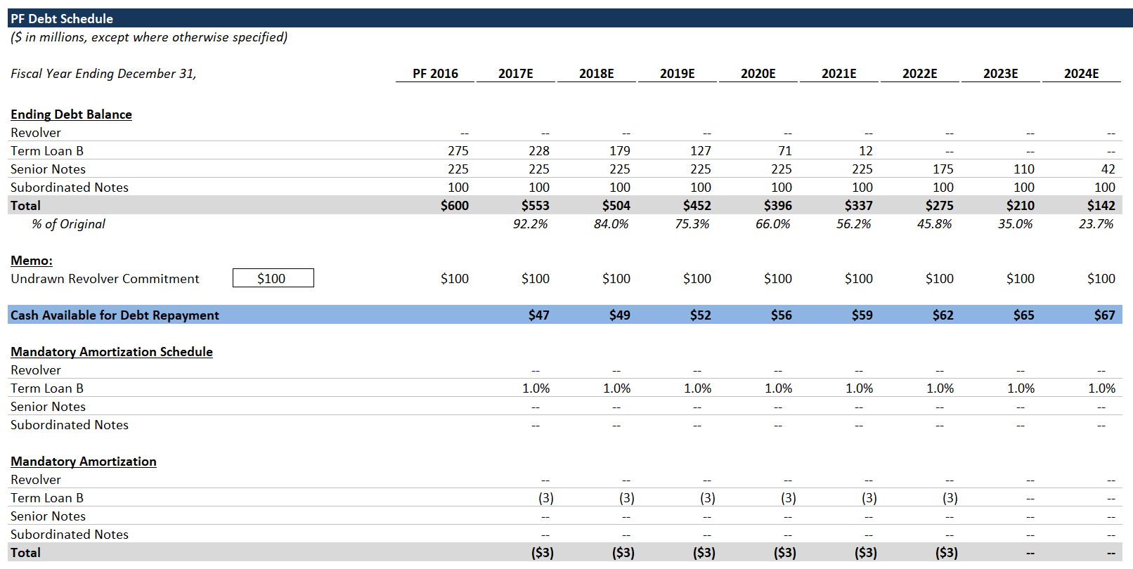
Note: typically, you can’t repay outstanding notes as soon as you’ve paid down the Term Loan B, as we’re doing here. Debt investors who buy high-yield bonds generally don’t want to be repaid early without a fee. If the company is doing well enough to repay the debt early, that means that the company is less risky, and investors would probably want to keep their capital deployed. Early repayment of notes is a simplifying assumption, and it’s typical to model LBOs this way. Alternatively, you could accrue a cash balance and/or refinance the notes.

12. Interest Expense Schedule

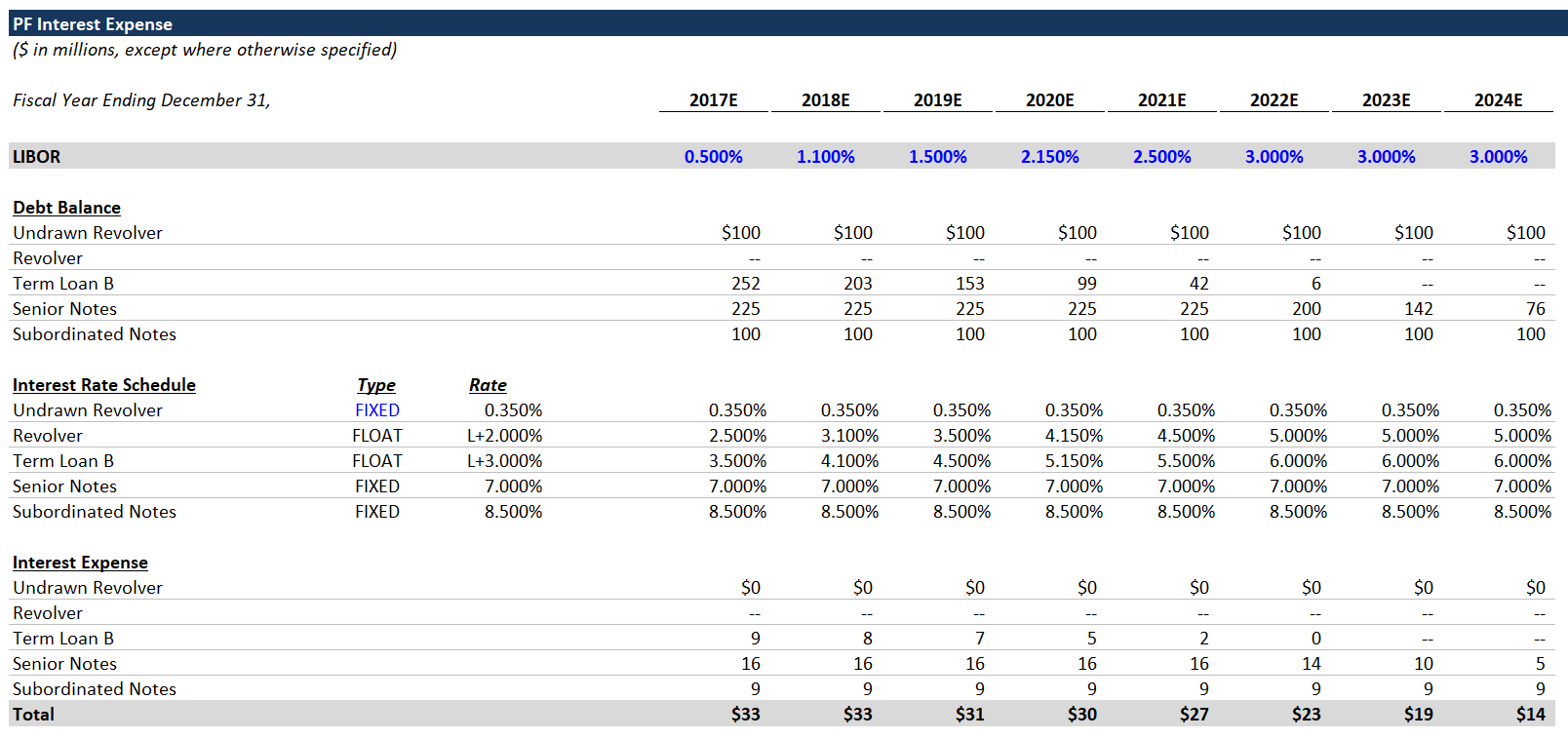
We’ve provided an illustrative LIBOR curve. If you’re unsure what this is, or what it’s used for, you should pause and read some of the debt primers provided at the beginning of this tutorial.

We include the Undrawn Revolver as a debt balance, because the company must pay a small amount of interest expense for the unused commitment.

For the Interest Rate Schedule, we’ve used a custom number format to achieve the “FIXED” vs. “FLOAT” formatting. You can google “Excel custom number format” to learn more. Here, where it says “FLOAT,” the cell value = 1, and where it says “FIXED,” the cell value = 0.

1. Calculate the debt balances. For each tranche, the debt balance should be the average balance from the beginning to the end of a given year. Use the following formula, similar to what we did when calculating Cash Interest Income:

   Debt balance = if (CIRC = 1, average(prior year balance, this year balance), prior year balance).
   If the circ switch is off, then the interest expense will be calculated using the beginning debt balance, which removes the circular reference.

2. Calculate the interest rate for each tranche.
   • For FIXED tranches, the interest rate should just be the stated rate.
   • For FLOAT tranches, the interest rate should be the sum of LIBOR and the stated rate. We could include more advanced functionality, such as a LIBOR floor, but it would be immaterial. You can read more about the intricacies of the various debt instruments in the primers.
3. Calculate interest expense for each tranche by multiplying the debt balance by the scheduled interest rate.
   • When the CIRC switch = 1, interest expense is calculated with the average debt balance.
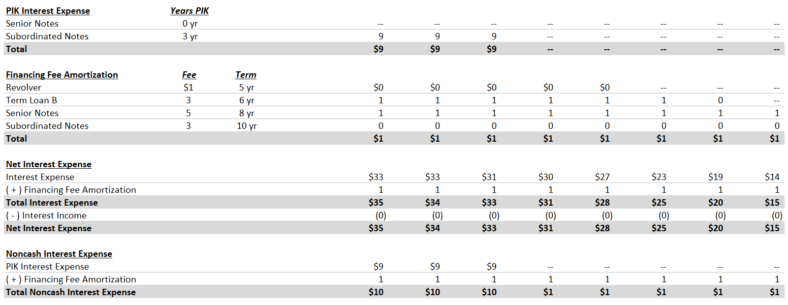
4. Next we’re going to calculate the “PIK” interest for the notes. For each year, compare the number of years elapsed to the PIK term, and if the number of years elapsed is less than or equal to the PIK term, we’ll include that debt tranche’s interest expense as PIK interest.
   • For the first 3 years, the subordinated notes “PIK.”
   • Since PIK interest is not paid in cash, it’s deemed part of noncash interest expense, which is added back in the statement of cash flows.

     Although Payment-In-Kind (PIK) interest is uncommon in the current financing environment, it pops up occasionally, and it’s an important concept to understand. When notes, or other debt, have a PIK feature, interest expense is not paid in cash for a number of years. Instead, the interest expense is added to the debt balance, so the debt balance accrues over time. PIK interest is a way for LBO investors to manipulate when cash payments occur. An investor might use a debt tranche with PIK interest expense to layer on additional debt, while keeping the interest expense manageable in the early years. The LBO investor would be counting on paying down more senior tranches of debt, alleviating some of the interest expense, before the PIK interest flips back to cash payment. This is an aggressive, riskier technique. Generally speaking, notes and mezzanine debt can have PIK interest. You can learn more about PIK interest here.

5. Calculate financing fee amortization - the other type of noncash interest expense. Capitalized financing fees are amortized over the life of the corresponding debt tranche. This annual amortization is included in Net Interest Expense, but is a noncash expense. Use the following formula:

   Tranche fee amortization = max(0, min(total fee - sum(prior amortization), total fee / debt term))

   • In English, take the lesser of (the total fee minus cumulative prior amortization) and the calculated annual amortization.
   • By locking the appropriate columns, you can drag this formula across all years and all tranches. Try to get it on your own, but compare with the completed sheet if you’ve having trouble.

Now we have all the components of interest expense. Interest Expense (including PIK interest) + Financing Fee amortization = Total Interest Expense; less Cash Interest Income = Net Interest Expense.

Likewise, we can calculate Total Noncash Interest Expense as PIK Interest + Financing Fee Amortization.

13. Putting the Pieces Together

Fixing the Debt Schedule

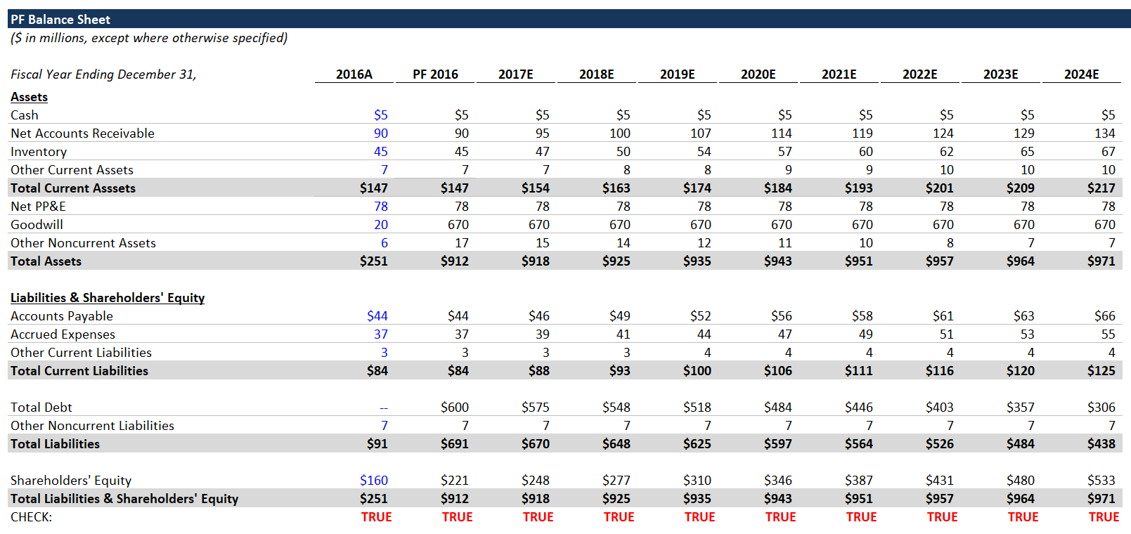
After calculating PIK Interest Expense, you may have realized we’re not properly accounting for it in the Debt Schedule. We’re going to fix that now. In the ending debt balance formula for the notes, add the corresponding PIK Interest Expense each year. For the first 3 years, the Subordinated Notes Ending Debt Balance should be increasing.

Adding Net Interest Expense to the Income Statement

Now, we’ll add Net Interest Expense to the Income Statement, and we’re going to include CIRC protection. This is redundant, because we already included a CIRC statement in our debt balance / Interest Expense calculation, but redundancy is better than debugging a broken model.

Use the following formula:

Net Interest Expense = if(circ=1, -Net Interest Expense from Interest Expense Schedule, 0)
Make sure you’re using net interest expense, which includes the Noncash Interest Expense and the Cash Interest Income.

Finalizing Statement of Cash Flows

Now let’s link Noncash Interest Expense into the Statement of Cash Flows as an add-back to Net Income. We do this, because Net Interest Expense reduces Net Income, but this portion of Net Interest Expense is a noncash expense. For the first 3 years, Noncash Interest Expense will be relatively high, because it includes the PIK Interest Expense.

Projected Balance Sheet

Next, we’re going to finish the Balance Sheet. The most important thing to remember when building out a projected Balance Sheet is that every line item in the Statement of Cash Flows must be reflected in the balance sheet. If there’s a single line item from the Statement of Cash Flows that is not properly incorporated in the Balance Sheet, your Balance Sheet won’t balance.

1. Link Cash & Cash Equivalents in each future year to the Ending Cash on the Statement of Cash Flows.
2. Link working capital line items from the Working Capital Schedule:
   • Net Accounts Receivable
   • Inventory
   • Other Current Assets
   • Accounts Payable
   • Accrued Expenses
   • Other Current Liabilities
     These line items are accounted for in the (Increase) Decrease in NWC line on the Statement of Cash Flows.
3. Keep Goodwill constant in all future years. Just set it equal to the prior year.
4. Keep Other Noncurrent Liabilities constant in all future years.
5. Shareholders’ Equity = prior year Shareholders’ Equity + Net Income.
6. Link Debt to the corresponding total debt balance in the Debt Schedule.
   • The changes in the debt balance include the following line items: Mandatory Amortization, Optional Prepayment and PIK interest (included in Noncash Interest Expense).
7. Other Noncurrent Assets = prior year balance - Financing Fee Amortization for the given year.
   • Now that we’re including Financing Fee Amortization, we’re fully incorporating the Noncash Interest Expense line from the Statement of Cash Flows.
8. Net PP&E = prior year Net PP&E + CapEx - D&A.
   • Basically, it grows every year by the amount of new capitalized assets less D&A. It’s constant here, because as a simplifying assumption, we’ve made CapEx = D&A.

The balance sheet should now balance, because we’re incorporating all line items from the statement of cash flows.

14. Credit Metrics

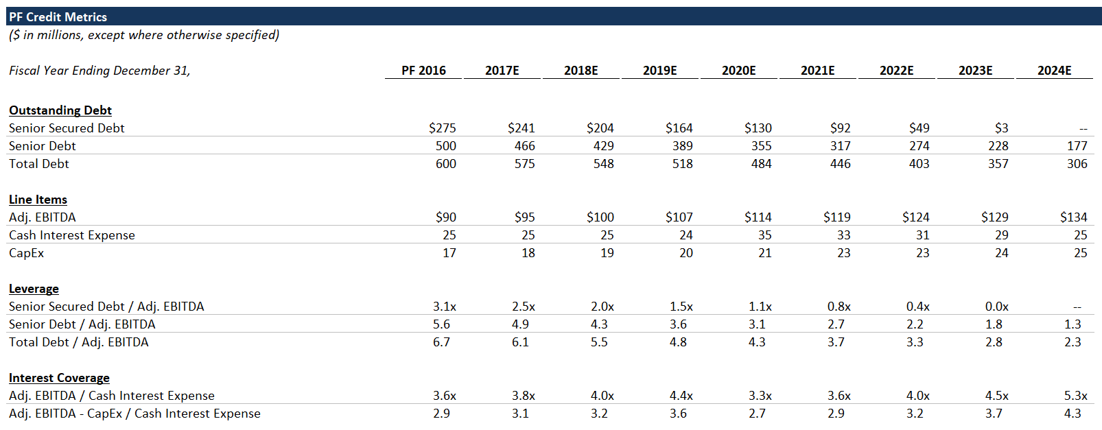
Every LBO model should include basic credit metrics, because these metrics and the credit profile will inform debt investors’ appetite to fund the transaction. They indicate the potential credit risk.

Credit Ratios
The two main types of credit ratios are leverage ratios and interest coverage ratios:

• Leverage ratios - compare the amount of debt and the company’s cash flow (EBITDA).
• Interest coverage ratios - compare the company’s cash flow (EBITDA) and the annual interest expense burden.

1. Link to the corresponding debt balances along with the EBITDA and CapEx.
   • Senior Secured Debt = Revolver + Term Loan B
   • Senior Debt = Revolver + Term Loan B + Senior Notes
2. Cash Interest Expense = Total Interest Expense (before Financing Fee Amortization and Cash Interest Income) - PIK Interest Expense.
3. For 2016 Cash Interest Expense, I generally set it equal to 2017 Cash Interest Expense as a shortcut. A better way is to calculate the full amount of Interest Expense (i.e., the starting debt balances multiplied by the applicable interest rates, less any PIK’d interest).
   • 2017 Cash Interest Expense should be lower than that amount, because debt is paid down over the course of the year, which leads to a lower average debt balance.
4. Fill out leverage and interest coverage ratios.
   • The ratios should be pretty self-explanatory, but refer to the completed sheet in case you have any issues.

15. Sponsor Returns

MoIC and IRR
When performing a LBO analysis, we measure sponsor returns using the Multiple of Invested Capital (MoIC) and the Internal Rate of Return (IRR). Sponsors get paid based on MoIC, but their investors care about IRR, so both are important. Even if a particular investment has a lackluster IRR, a decent MoIC is good for the sponsor, because they get a share of the dollar profits (not based on IRR). That being said, the fund IRR will be important for marketing their next fund to investors.

MoIC is literally the multiple of money made, e.g., the sponsor and its investors made 3x their money. IRR is the discount rate that would be required in order for the sponsor to achieve a $0 NPV from the investment. These are closely related concepts - the difference is that IRR takes into account the timing of cash flows, whereas MoIC measures only the dollars. You can Google to learn more.

Exit Multiple Sensitivity
Using line items from the rest of the model, and a range of exit multiples, we’ll calculate the sponsor’s returns (MoIC and IRR). Showing a range of exit multiples is helpful, because it highlights the impact that the exit multiple can have on returns. PE firms often hold investments 5+ years, and the valuation of a particular asset can shift dramatically over that time frame. In the best case scenario, the sponsor buys an asset at the bottom of the cycle, and valuations subsequently skyrocket. An exit multiple that’s substantially higher than the entry multiple is a great way to make money, but the opposite can happen, too.

When a sponsor sells an investment for an exit multiple that’s higher than the entry multiple, that’s called Multiple Expansion. It’s an elusive, mythical beast, and you can read more about it here.

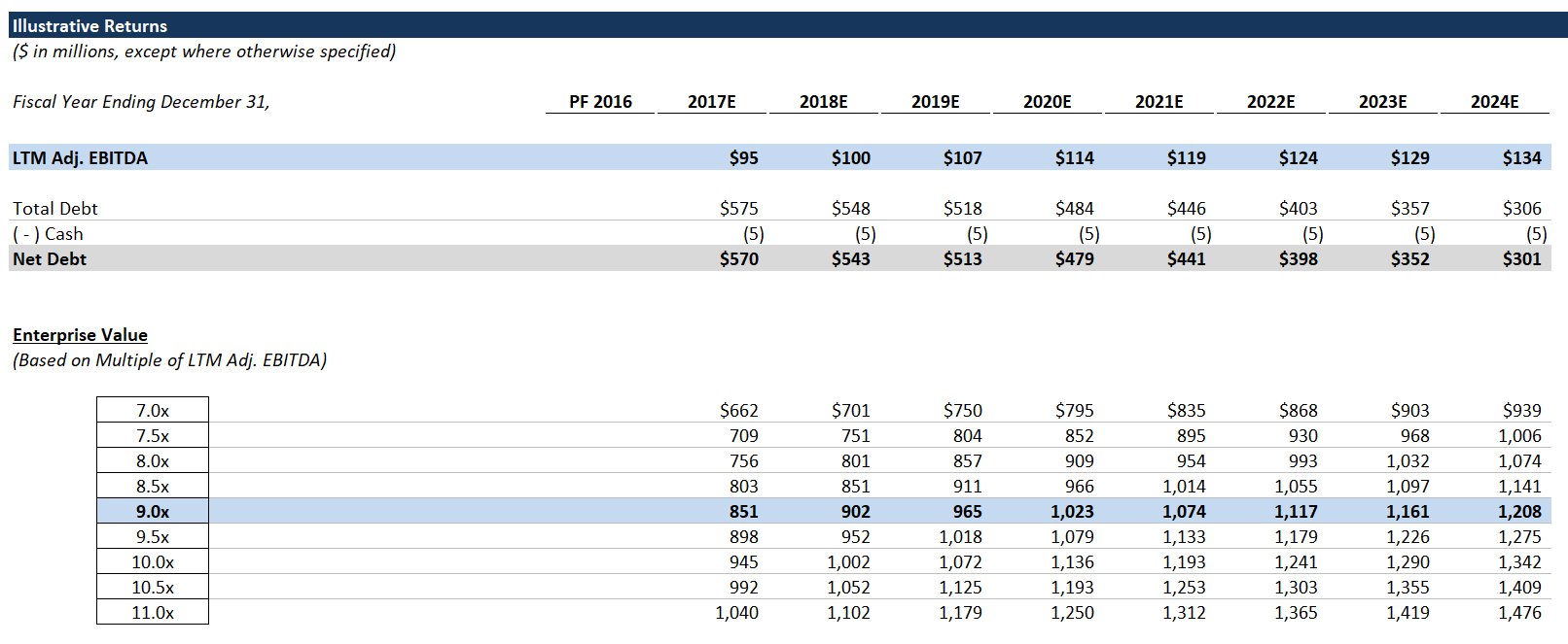
1. Start by linking Adj. EBITDA, Debt and Cash.

2. Calculate Net Debt.

3. Calculate Enterprise Value based on the exit multiples on the left (Enterprise Value = exit multiple x LTM Adj. EBITDA).

   • The highlighted row corresponds to the entry multiple (i.e., constant entry and exit multiples).

4. Equity Value = corresponding Enterprise Value (which varies by exit multiple) - Net Debt.

5. Set Investment equal to the total equity invested: Sponsor Equity + Management Rollover.

   • In a real transaction, there would be a complicated split of investment proceeds between management and the PE firm. A higher-level analysis, like this one, generally just lumps them all into one bucket.

6. Calculate MoIC by dividing Equity Value by Investment.

7. Above the IRR section, add a row for the number of years elapsed. This will make it easier to calculate the IRRs. You can enter the years elapsed manually or you can use the Year function:

   Years Elapsed = Year(current column date) - Year(PF 2016 date).
   (You can refer to the date row at the top of the returns schedule).

8. Calculate IRR with the following formula:

   IRR = MoIC ^ (1/ Years Elapsed) - 1

Next Steps

Congrats, you’ve completed the training LBO!

Try the rest of our private equity modeling tutorials:

1. Ability-To-Pay Analysis
2. LBO Value Creation
3. Dividend Recap Guide
4. Advanced LBO Modeling
5. Private Equity Modeling Guide