Introduction

This is going to be a shorter post. We’re going to explore the concept of unit economics - what it means, why unit economics are important, and a few examples.

I struggled to understand unit economics for an embarrassingly long time. I heard the term used in management presentations, by investors, by my bosses, and I never really got it. Oh yeah, the unit economics. Of course.

My hope is that this article will cure you of this problem or, if you’re already familiar with the concept, improve your understanding. So here goes.

Definition

The term unit economics refers to the base unit of activity for a given business and the profitability / economics of that unit. Let’s break that down.

Unit economics consist of two conceptual pieces:

1. the base unit of activity and
2. the economics or profitability of that unit.

Base Unit of Activity

The base unit of activity for a given business is the smallest logical piece that helps you understand the business as a whole.

Below are some examples:

• For a retail company, like J.Crew, the smallest unit of business is an individual store.
• For an ecommerce company, like Amazon, the smallest unit of business is an individual online purchase (could consist of multiple items).
• For an ocean shipping company, with a fleet of ships, the smallest unit of business is an individual ship.
• For an upstream oil & gas company, the smallest unit of business is an individual well.
• For a home builder, the smallest unit of business is an individual home.
• For a SaaS business, the smallest unit of business is a subscription.
• For a power generation business, the smallest unit of business is a power plant.

Choosing the base unit(s) of activity requires some discretion. You must disaggregate how many base activities the company is engaged in. For example, many retailers are working to strengthen their ecommerce operations. You might choose to evaluate such a company as two separate businesses: (i) a physical retailer and (ii) a supplemental ecommerce business. The base unit of the retailer would be a single store, and the base unit of the ecommerce business would be a single transaction.

Likewise, maybe an oil and gas company is involved in two separate plays, each with its own well profile. Or perhaps a retailer has multiple distinct store formats. You might choose to evaluate each format as its own business line, with its own unit economics.

Profitability / Economics

The second step is understanding the economics for the selected base unit(s) of activity. You need to understand the revenue & expense drivers:

• What variables determine revenue? What do they depend on?
• What variables determine expenses?
• How fixed / variable is the cost structure?

You also need to understand any CapEx associated with the unit:

• Does this base unit require a big investment to build / bring online?
• How long does it take?

For example, power plants take a long time and a lot of money to build. But for the marginal software subscription, there’s no cost, and it could be instantaneous.

Unit economics encompass all the variables and information needed to build a simple financial model for the base unit(s) of activity.

Let’s look at some examples.

Retail

Financial drivers for a store:

• Sales per sq. ft. ($)
• Store size (sq. ft.)
• Build-out cost
• Rent, financing & other fixed costs
• Gross margin

Ecommerce

Financial drivers for a transaction:

• Transaction size ($)
• Gross margin
• Any attributed marketing spend (e.g., online ads)

Ocean Shipping

Financial drivers for a ship:

• Utilization percentage: what % of time is the ship under contract?
• Average fee / contracted day
• Fuel & other variable costs
• Maintenance costs & schedule
• Rent, financing & other fixed costs

Upstream Oil & Gas

Financial drivers for a well:

• Forecasted production curve (volume)
• Opex
• Capex
• Transport costs
• Oil / gas price

Software as a Service (SaaS)

Financial drivers:

• Churn / expected customer lifetime
• Customer acquisition cost (CAC)
• Price
• Any variable costs associated with subscription (e.g., dedicated support rep)

Power Generation

Financial drivers for a power plant:

• Forecasted production (volume)
• Price
• Variable production costs
• Maintenance costs & schedule
• Cost to build & timeline
• Financing & other fixed costs

Why Unit Economics Are Important

Unit economics help us think about the profitability and growth potential of a business.

Going back to our examples, a retail company is really just the sum of all its stores and some corporate overhead. Likewise, a shipping company is the sum of all its ships and some corporate overhead. You get the idea. Understand the part, and you understand the whole.

Furthermore, unit economics simplify a complex problem by providing a smaller surface area to examine. Forget the overall company - how profitable is one store?

If a company’s unit economics look great, but the overall financial profile is lackluster, that sounds like an investment with potential for improvement (and opportunity for multiple expansion).

If a company’s overall profile is fine, but the unit economics are rapidly degrading, that’s cause for alarm.

In Practice

Unit economics are an important tool for investors.

Private Equity

In private equity deals, a company’s unit economics are one of the major diligence items. If the unit economics look bad, that’s a dealbreaker!

Venture Capital

Since venture-funded businesses do not have much of a track record, understanding the unit economics and potential market size are crucial.

Public Markets

Investors try to determine the health of companies’ unit economics from public filings and other publicly available data. Understanding the unit economics is a key step in researching industries and forming a thesis.

Introduction

This article will explore and explain some first principles of capital structure and how capital structure impacts returns. In many conversations with (junior & senior) finance professionals, we have heard “leverage” referred to as a cure-all.

• “Leverage will help with that.”
• “Let’s add some leverage and juice the returns.”

We want to help you develop a better intuition for capital structure and how leverage really works.

What is capital structure?

Capital structure is the sum of all the different types of capital supplied to a particular asset or company. Capital just means financing. Where is the money coming from - and in what form? For example, if you buy a house with a mortgage and some cash down, the house’s capital structure consists of the mortgage (debt) and your cash down (equity).

The same logic applies to companies. Let’s look at a few examples:

Early-stage Software Company
It’s a startup, baby! (100% Equity)

Early-stage software companies are usually financed entirely with equity (no debt). The equity, however, may be broken into multiple tranches (e.g., preferred vs. common), some with priority over others.

Industrial Manufacturing Company
Plain Vanilla Co

An industrial company could support some debt in addition to equity. Where it sources that debt from depends on the size of the company. Smaller companies might get a secured loan from a regional bank. Larger companies might tap the capital markets (and an investment bank) to raise public debt.

Ocean Shipping Company
Fixed Assets with Resale Value

A shipping company might have equity stakes in multiple large ships. These ships will be financed partially with secured debt (the debt has recourse on particular ships, like a mortgage). In addition, the shipping company might have unsecured, company-level debt. The company is also financed with equity.

These are just a few examples.

Capital structure varies greatly across - and within - industries

For this article, we are not going to focus on specific types of capital (e.g., secured debt, bonds, preferred equity, etc.). These are just labels that have evolved by convention to define certain scenarios. The more important takeaway is that capital structure and specific forms of capital vary greatly and are only limited by two factors:

1. Human ingenuity
2. The market’s willingness to fund a particular instrument / opportunity (at a given price)

Why does capital structure vary?

First, there are industry norms and company life cycle considerations.

Industry Norms

Industry characteristics have a major impact on capital structure. Below are a few example factors:

• How capital-intensive is the industry? Some industries (e.g., real estate, natural resources) require lots of capital.
• Do companies have fixed assets? Fixed assets offer a measure of safety / security to investors.
• How predictable is the revenue?
• How does the industry fair in a downturn? Resilient revenue is always a plus.

All these factors (and more) help define capital structure norms for a given industry.

Company Life Cycle

A company’s life stage can play an important role as well. For example, a startup will not be able to raise institutional debt. Smaller, younger enterprises are inherently riskier and unproven, and therefore, only certain providers of capital have appetite to fund them.

On the other hand, mature enterprises will not seek venture capital and other expensive forms of capital, because they have access to cheaper sources, such as public equity and debt markets.

Strategy & Management

Finally, different management teams will pursue different capital structures as part of their overall strategy. So even within a homogenous industry, capital structure varies.

First Principles

Now, let’s establish some first principles.

1. A given company can have an indefinite number of tranches of capital. There is no theoretical limit on the number of different tranches / sources of capital.

2. These tranches of capital are arranged in order of seniority (most senior to least senior).

Seniority refers to the order in which the tranches of capital are paid in a liquidity event. For example, if a company were sold, the senior debt would be paid off first, then the junior debt, then the preferred equity, and then the remaining proceeds would go to the common equity.

Therefore, the most senior tranches are least risky, and common equity is riskiest.

3. Riskier tranches of capital demand a higher return. Risk and reward are dear friends.

Investing is the art of identifying temporary dislocations in the pricing of risk. For example, if the market is pricing a certain risk higher than you think it deserves (granting it an outsized return), you can buy that opportunity and pocket the extra return.

4. Each successive tranche is riskier than preceding tranches, since each successive capital tranche is junior to the preceding tranches.

5. Therefore, each successive tranche demands a higher rate of return than preceding tranches.

Of course, the very bottom of the capital structure is common equity. It represents the claim after all other tranches (debt & equity) have been fully serviced.

Returns

Cool, enough chitchat. How does all this factor into returns?

To answer that question, let’s start with the simplest possible capital structure:

100% Equity

The company is funded entirely with uniform equity (only 1 tranche). How do we calculate the equity return?

In this instance, the Return on Equity (ROE) equals the Return on Assets (ROA). Because there’s no leverage or any other tranches. For example, if the ROA = 10%, the ROE = 10%.

The Return on Assets (ROA) is the unlevered return to the enterprise. You can calculate it as the company’s unlevered cashflow / net operating assets (total assets, but accounting for items like negative net working capital).

Note: there are many variations on how to precisely calculate the ROA and what the proper numerator (in the fraction) is. For this conversation, these variations are not important. You just need to understand that it represents the unlevered return on the company’s assets.

Okay, let’s add some leverage.

50% Debt, 50% Equity

In this scenario, let’s assume the following:

• ROA = 10%
• 50% debt, 50% equity
• 100 total invested capital
• 5% tax-effected cost of debt

What’s the return to shareholders (ROE)?

Total ROA: 10 (10% x 100)
Cost of debt: 2.5 (5% x 50)
Return to shareholders: 7.5 / 50 (15% ROE)

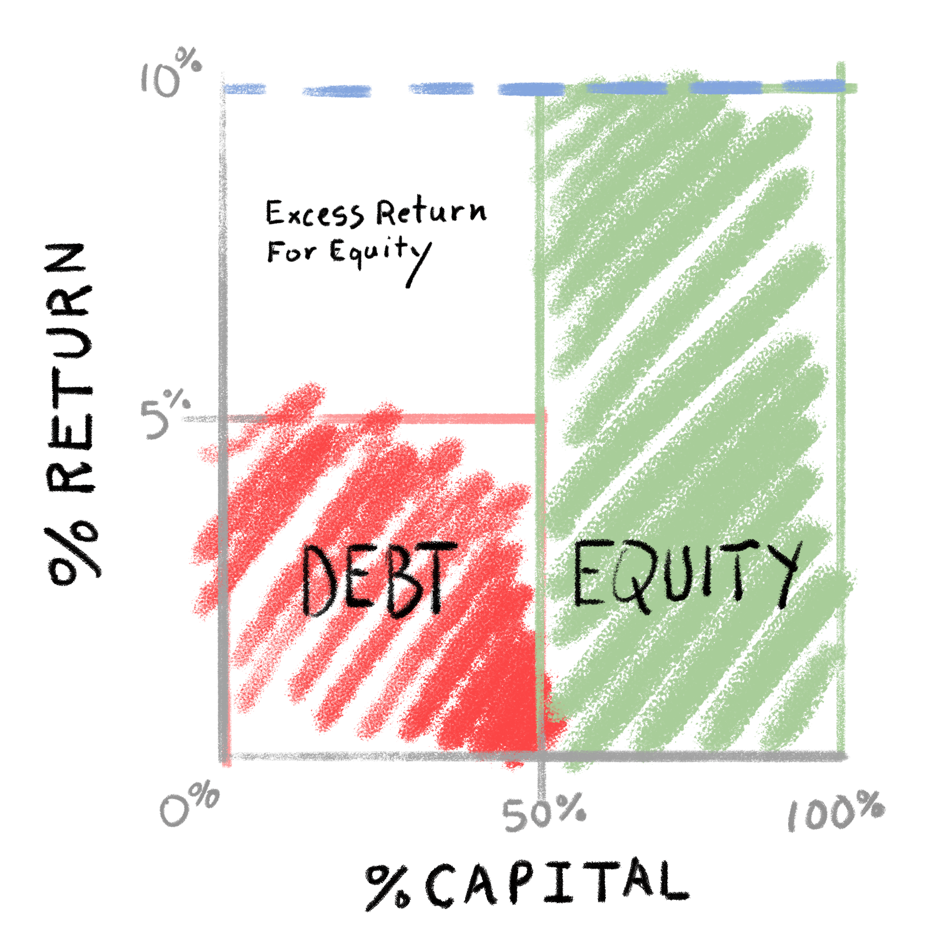
So leverage juiced the return to shareholders by 50%! I think a graphic is the most intuitive way to understand this. See our scenario below:

As you can see, equity receives the sum of:

1. the ROA multiplied by the amount of equity
2. all of the remaining ROA after other capital tranches have been serviced

   1. 10% ROA x 50 equity = 5
   2. (10% ROA - 5% cost of debt) x 50 debt = 2.5
      ROE = 7.5 / 50 equity = 15%

Leverage, however, also increases the risk to shareholders.

In the scenario below, where the ROA drops to 4%, equity returns dry up. Recession ain’t fun.

What’s the return to shareholders (ROE)?

Total ROA: 4 (4% x 100)
Cost of debt: 2.5 (5% x 50)
Return to shareholders: 1.5 / 50 (3% ROE)

Now, let’s examine a more complex, but realistic scenario.

35% Secured Debt, 35% Notes, 30% Equity

Let’s assume the following:

• ROA = 10%
• 35% secured debt, 35% unsecured notes, 30% equity
• 100 total invested capital
• 4% tax-effected cost of secured debt
• 8% tax-effected cost of unsecured debt

What’s the return to shareholders (ROE)?

Total ROA: 10 (10% x 100)
Cost of secured debt: 1.3 (35 x 4%)
Cost of unsecured debt: 2.6 (35 x 8%)
Return to shareholders: 6.1 (20% ROE)

Here’s the chart:

As you can see, these leverage assumptions take an asset yielding 10% to PE-salivating equity returns. This is the magic of leverage.

This scenario also illustrates our first principles.

1. We have multiple tranches of capital.
2. Secured debt is most senior, then notes, and finally equity.
3. Riskier tranches have a higher cost of capital.
4. Each successive tranche is riskier.
5. Each successive tranche is more expensive.

Other Takeaways

Leverage = Risk

We can use this logic to screen investments. For example, if we’re evaluating opportunities in a given industry and we come across two companies with similar equity return profiles, but one is more levered, choose the company with less leverage (all else being equal).

Our first principles tell us why: For a similar return, with the levered company, we would be assuming more risk. Remember - equity comes at the bottom of the capital structure.

Second Principles

The charts we’ve used to illustrate these scenarios reveal a few final principles:

1. If the cost of incremental capital is less than the ROA, the incremental capital will increase the ROE - and, of course, the risk to common equity.

We can see this clearly from the third chart. Common equity receives the surplus region between the ROA and the cost of capital for all other tranches.

2. Conversely, leverage will only hurt the ROE once the ROA drops below the cost of capital for one of the preceding tranches.

Therefore, it is in shareholders’ best interest for companies to raise debt and buyback shares as long as the cost of debt is significantly below the ROA (i.e., even in a recession, the ROA wouldn’t dip below the cost of debt).

3. Lastly, a company should not raise capital, when the cost of capital exceeds the ROA. Such financing would decrease the return to shareholders (ROE).

Note: One potential exception to these principles would be a company raising outsized debt in order to fund a transaction - and then paying off the debt ASAP. In some LBOs, the sponsors have been quite aggressive and raised expensive debt with the goal of paying it down or refinancing it within the first few years. Obviously, this greatly increases the risk as well.

Introduction

When you finish your LBO model and calculate a juicy IRR, that feels good. But what does that IRR represent? How much money is the sponsor making vs. the management team? How does that split change based on the success of the deal?

This post will strive to address these questions. But - if you haven’t worked through our preceding private equity tutorials (listed below), please review those first.

1. Easy LBO
2. Intermediate LBO
3. Ability-To-Pay Analysis
4. LBO Value Creation Analysis

High Level

Essentially, we’re talking about the equity waterfall, which is the division of equity proceeds amongst all the different equity holders.

You may have thought that equity was just one amorphous blob, where everyone is equal – I know I did at first. That is not the case. The division of proceeds amongst different classes of stock and investors can be as tricky as debt waterfalls (for more on debt waterfalls, check out our Intermediate LBO Guide).

OK, if the equity waterfall is so nuanced, why do most banker LBO models treat all shareholders the same? Because the division of equity proceeds is bespoke to each deal, and frankly, treating all shareholders as one unit is a good approximation. For a pitch, you generally just want to know if the sponsor returns pass the smell test (minimum 20% IRR for a vanilla financial sponsor).

Takeaway: For bankers, the equity waterfall for a private equity deal usually doesn’t matter. It is crucial, however, for the financial sponsor and their partner management team.

Why is the equity split bespoke?

For each private equity deal, management’s compensation package (and the equity split) is heavily negotiated. Many different factors can influence these negotiations; below are some of the most important considerations:

Relative value of the management team

• Are they the best in the industry, or just hoping to keep their jobs?
• Can the asset be operated without this team?
• Would the sponsor do the deal without this team?

Sale process dynamics

• How many other credible sponsors are bidding?
• Is this a must-sell-now situation, or can the seller afford to wait if no amenable bids come along?

PE firm size / culture / social issues

• How large is the private equity firm?
• How flexible is the private equity firm?
• How junior is the partner leading the deal?

Influenced by these variables, and many more, the sponsor and the management team will negotiate an equity package - basically, management’s piece of the pie. This will form the bulk of management’s total compensation, and it will be structured to align incentives.

The sponsor wants to keep management’s compensation as low as possible, while (a) maintaining a cordial and productive working relationship and (b) incentivizing the team. Meanwhile, management wants to grab as much equity as they can.

Example Equity Waterfall

Here is the completed Excel file, which builds off of our preceding tutorials. We’ll be discussing the Equity Waterfall tab.

Key Assumptions

• Single sponsor deal
• Sponsor uses preferred stock with an accruing hurdle rate
• Preferred stock converts to common on a 1-1 basis
• Management compensation structured with stock options

Let’s discuss each of these in more detail.

Single sponsor deal

There are no coinvestors or other complicating factors. This is about as simple as it comes (one sponsor partnering with a management team).

Preferred stock with a hurdle rate

• Sponsor uses preferred stock to protect against downside risk. Preferred stock is senior to common equity, so if the deal goes sour, the sponsor would be paid in full before the management team.
• Hurdle rate allows the sponsor to accrue some minimum return threshold (essentially, before the management team is paid). This feels a little nasty, but you can understand the rationale: if the sponsor only makes a 2% return, the management team did a bad job and shouldn’t get paid.
• Here, we’re assuming an 8% hurdle rate.

Convertible preferred

• The preferred stock is convertible to common stock. If the deal goes well, the sponsor can convert its preferred stock to common stock and share in the upside.
• Also, since the sponsor has been accruing the hurdle rate, the sponsor receives more common stock than its initial investment would warrant.

Stock options

• We’ve structured management’s compensation using a series of stock options with progressively higher strike prices. As the exit value increases (successful deal), management gets a bigger piece of the pie.

Enough chitchat, let’s review the actual model.

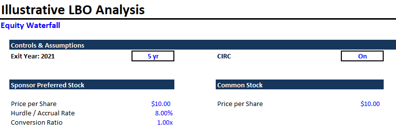
Controls & Assumptions

We don’t have many controls and assumptions.

A couple things to point out:

1. You can change the exit year, to see how the payout changes for different holding periods.
2. You can change the preferred acrrual rate and the conversion factor.

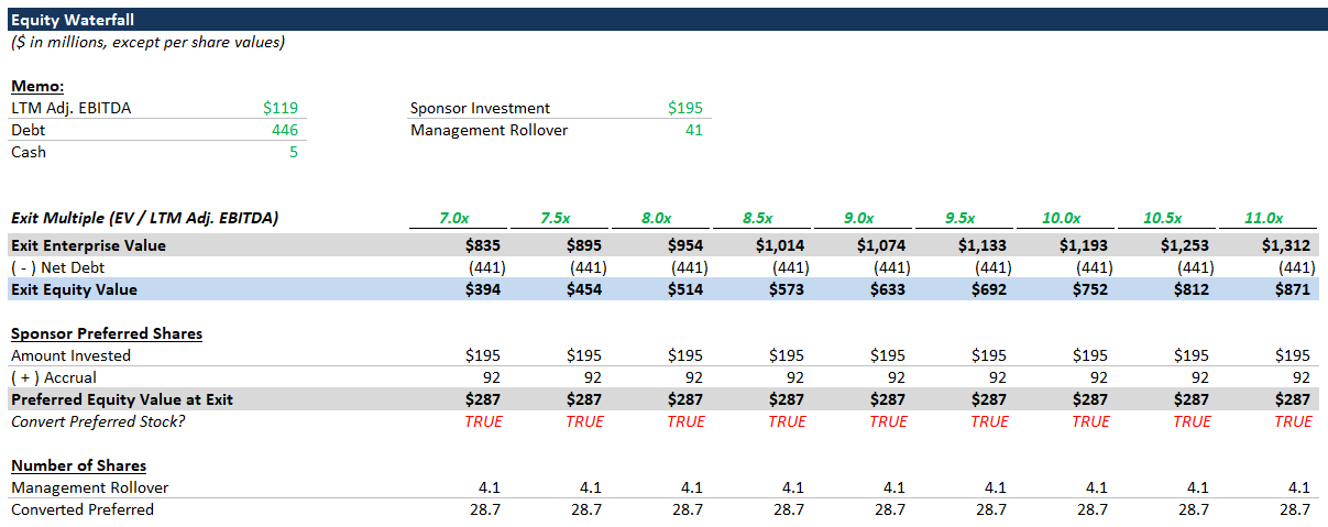
Equity Waterfall (part 1)

The top of the equity waterfall shows our build to equity value and calculates the value of the sponsor’s preferred stock (including the accrued hurdle rate). The sponsor will only convert the preferred stock if the value of received common stock is greater.

Here, we’re making a simplifying assumption that the sponsor converts as long as the total equity value is greater than the accrued preferred stock. Note: the mechanics of the conversion right would be negotiated.

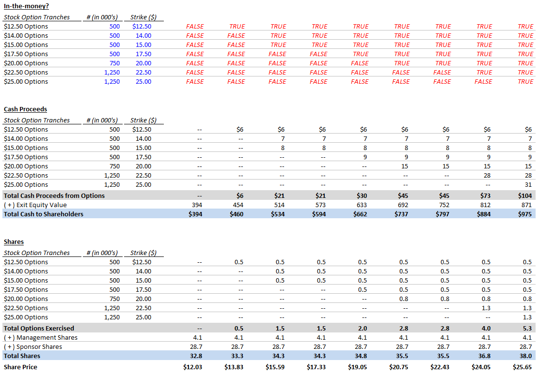
Equity Waterfall (part 2)

The remainder of the equity waterfall handles the management team’s stock options. We’ve structured 7 different tranches of options with progressively increasing strike prices. This aligns management’s incentives with the sponsor’s - management gets paid more as the sponsor makes more money.

You’ll notice that we add the option proceeds to the equity value. This is different from the treasury stock method, but it follows a similar logic. The money paid to exercise stock options becomes available to all equityholders, thereby increasing the equity value (whereas the treasury stock method assumes that the cash used to exercise options is used to repurchase shares).

As you’ve probably guessed, this creates a circular reference: The implied share price is based on the total number of shares, which includes exercised options, which in turn depends on the share price.

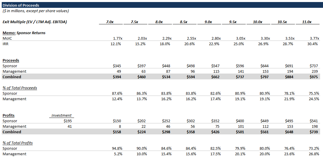
Division of Proceeds

Here, we calculate the sponsor’s returns: (i) IRR and (ii) Multiple of Invested Capital (MoIC). These return figures are different from those at the bottom of the LBO tab, because these figures isolate the sponsor’s returns vs. the aggregate shareholder returns.

The more important part of this section, however, is the division of proceeds and profits between management and the sponsor. You’ll notice that management’s split forms an upward-sloping curve - as the exit value gets higher, management gets a bigger piece of the pie.

This division of profits is a key negotiation point between the sponsor and management. The sponsor relies on the management team’s strategic plan and expertise to form projections for the business. Those projections are then used in the sponsor’s financial model to project returns. The sponsor also uses these projections when negotiating management’s compensation package. They essentially tell the management team: Hey, if you achieve your stated financial plan, you’ll be well paid.

Hence, the saying that management always sandbags their numbers - to manage expectations and get paid!

Introduction

Excel data tables are pretty sweet, right? They enable you to perform sensitivity analysis with minimal effort. (For those of you who haven’t dealt with Excel data tables before, here’s a quick primer). For those of you enamored with data tables, I’ve got bad news: you could be doing it better.

If you’re doing something quick ‘n’ dirty, Excel data tables are okay. For anything more complicated, or any analysis that will be a recurring piece of your project / presentation, you shouldn’t use them.

This article will show you a better way to perform sensitivity analysis - leading to clearer, more auditable models.

Background Articles

This article will build off the prior two articles, so if you haven’t worked through those, please go to square 1.

1. Accretion Dilution 101
2. Adding Flexible Cases to a Financial Model

Why not data tables?

Below is a summary of the main problems with data tables.

Hard-codes

Variables sensitized using Excel data tables must be hard-coded. Oftentimes, however, the variables that you want to sensitize in a data table are the same variables you would like to include in your cases (covered in the prior article - #2 in the list above).

In the short-run, this isn’t a dealbreaker. You can replace the linked variable with a hard-code, then run the data table, paste your outputs to PowerPoint, and then finally relink the variable. In the long-run, however, this becomes quite tedious, especially when sensitizing multiple variables. Furthermore - late at night, under time pressure - you are more likely to forget one of these steps and make a mistake. Perhaps a subset of the outputs you pasted to PowerPoint are wrong - hopefully, you catch the mistake and just have to repaste.

Worse case: you wake up to a nasty email from your MD.
Worst case: you send a wrong output to the client and get called out.

Switching back and forth between hard-codes and linked variables is not a good system.

Slow AF

When you’re working on a bigger model and add multiple data tables, you will notice a slowdown. Even if you set calculations to manual vs. automatic, data tables cause a big performance hit.

Auditability

How do you audit a data table? If it’s a two-way data table (most common), you have to manually set the two variables (in your model) and then trace through all the logic to confirm that everything is working properly. This is tedious at best, and has the same drawbacks discussed above under Hard-codes.

Self-Referencing If Statements

That’s a mouthful, huh? Stay with me. Self-referencing if statements are a thing of beauty. Self-referencing if statements are one of those tells that separate a great financial modeler from a competent one.

Definition

A self-referencing if statement is an if statement that references itself. Here’s a simplified example:

cell = if(criteria, exterior value, this same cell)

What’s going on here?
Basically, if the given criteria is True, show the linked exterior value; if not True, then just show the value already displayed in this cell.

Another way to think about it is a snapshot. If the criteria is True, take a new snapshot. If not, just show the last snapshot.

Cool story - why do we care?

Building off the last article (which showed how to construct cases), we can combine cases with self-referencing if statements to build better sensitivity tables.

Here’s a simplified example:

We’re creating a sensitivity table for a merger model. We’re showing how the % accretion changes as a function of the % offer premium and % stock consideration.

Step 1: We can create a case for each data point in the sensitivity table. Ex:
20% premium w/ 25% stock, 50% stock, 75% stock
25% premium w/ 25% stock, 50% stock, 75% stock
…
40% premium w/ 25% stock, 50% stock, 75% stock

Step 2: Create the sensitivity table output. Instead of a traditional data table, in each cell we’ll use a self-referencing if statement.

cell = if (RUNNING CASE = THIS CASE, model accretion, this cell)

How does this work?

Only the running case updates. The numbers for all other cases are frozen until you change the running case.

If this is still confusing, don’t worry. We’re going to work through a real example below.

This is dope

Data tables built with self-referencing if statements solve the issues we have with traditional data tables.

Fewer hard-codes

Your data tables automatically update as you change cases. The only hard-codes are the referenced case numbers. You don’t have to switch back and forth between hard-coded and linked variables.

Need for speed

Self-referencing if statements don’t hurt performance. Intuitively, this makes sense. All cases, except for the running case, are frozen.

Auditing has never been easier

Each data table cell links to the same calculated number in your model. To audit a given case or cell, just update the running case.

Real Example

Now, let’s work through an example. We’re starting with the completed Excel template from the last article. For reference, here is this article’s completed template, but we suggest working through the steps below.

Offer Premium & Consideration Mix

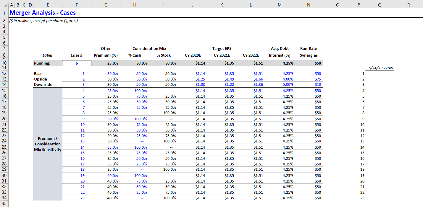
1. Go to the MCASE tab. As you can see, we’ve already created the cases for you. We’ll be looking at % accretion as a function of % premium and % stock consideration.

2. Let’s name the Running Case cell (F10): MCASE.

   Naming Cells
   You can name a cell by highlighting the given cell and pressing CNTL + F3. Then select New, and enter the cell name.

   Naming cells makes it easier to refer to them in different sheets. Now we’ll be able to refer to the running case as MCASE.

   NOTE: use this Excel feature sparingly. A little bit goes a long way.

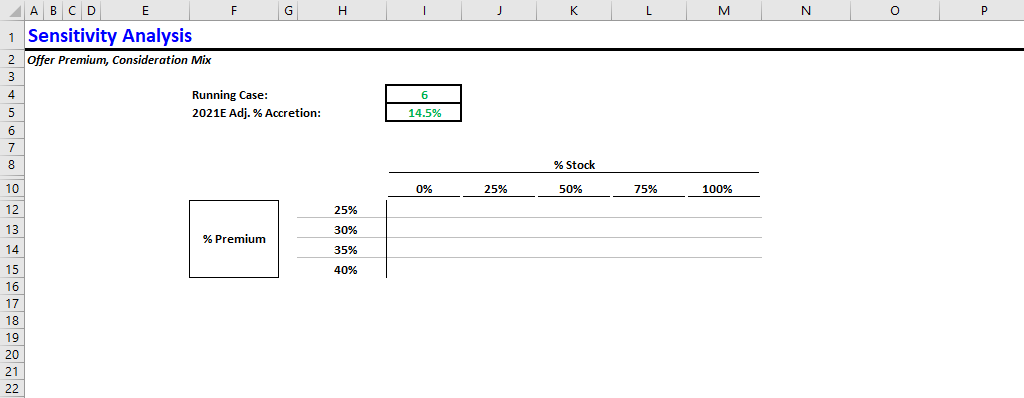
3. Now let’s create the sensitivity output. Create a new tab called - you guessed it - Sensitivity. Then create a skeleton of the % accretion sensitivity table.

Here’s what ours looks like, but you can format it however you like.

NOTE: we like to include the financial item being sensitized, so that the data table cell formulas don’t have to reference another tab, but that’s just personal preference.

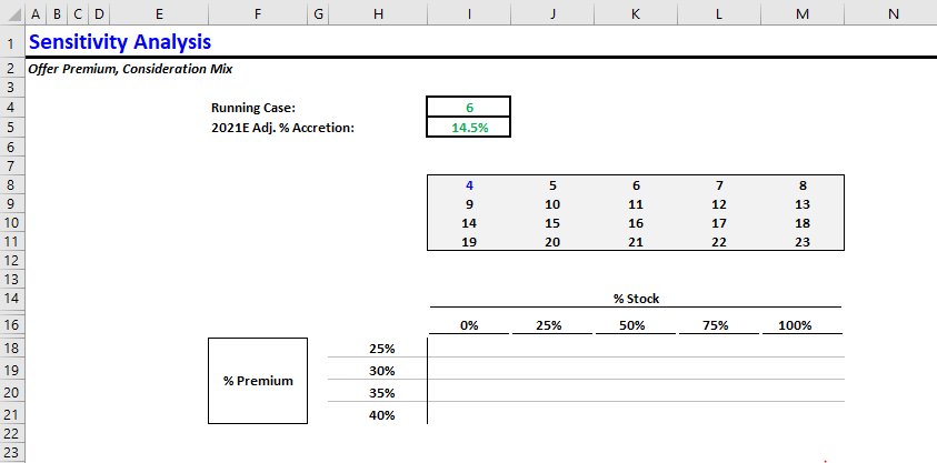
4. Next, let’s add the relevant case numbers in a box above the data table. If you’re not sure what I mean, see below. If you go back to the MCASE tab, you will notice that each case (4 - 23) corresponds to one of the data table cells.

5. Time to add the actual calculations. Remember the formula:

   this cell = if(MCASE = case number, % accretion, this cell)

Try your best to apply the formula, but you can reference the completed sheet if you get stuck.

NOTE: If you get a circular reference warning, you need to enable iterative calculations. Google if you’re not sure what this means.

6. If you implemented the formula correctly, only one of the cells in the table should have updated. The rest should be 0. Why? Because we’ve only run one case so far (the current case). Go back to the MCASE tab and run cases 7 and 8. On the Sensitivity tab, you’ll see a couple more cells updated.

As you’re probably thinking, manually running every single case would be super tedious. Fortunately, we have a solution for that. Get ready for some Excel magic.

7. Go back to the MCASE tab. To the right of your case variables, leave a blank column for spacing and then add two new columns. Set the first column equal to the row’s case number. Leave the second column blank, but at the top (above all case numbers), set a cell equal to the current date.

   cell = now()

Here’s what that looks like.

8. Now, we’re going to use an Excel data table to run all cases automatically. I know, I know. Data tables are bad, but this is one place where you need them. Typically, my workflow is:
   i) Build model
   ii) Design outputs
   iii) Run cases (via data table)
   iv) Delete data table (so model doesn’t lag)
   v) Paste outputs

If you need to run the cases again (i.e., to repaste), it’s easy enough to reinsert the data table, and then delete it.

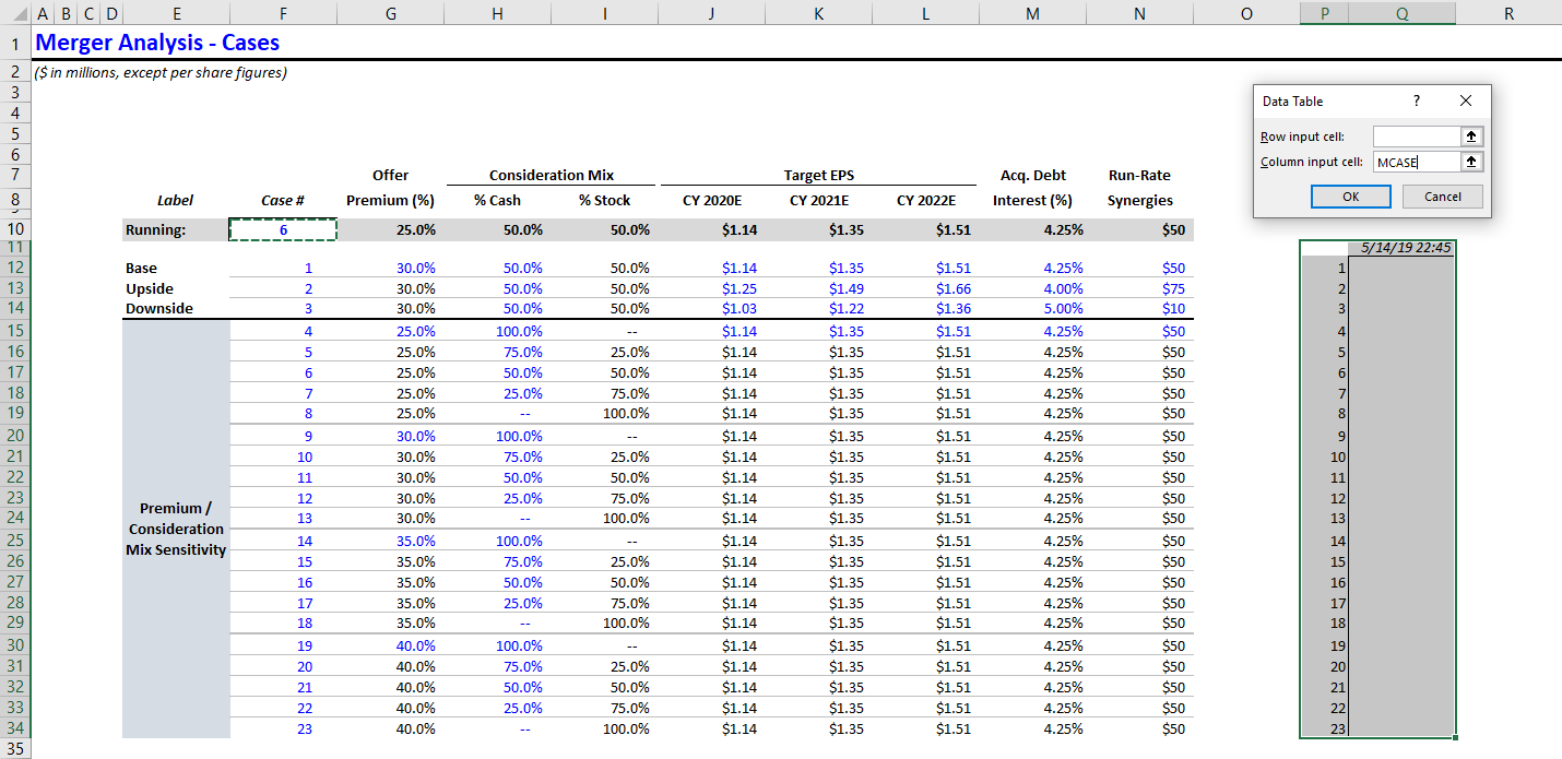
Ok, so let’s add that data table. Highlight the two columns you added (the case column and the empty column with the date on top). Then create a one-variable data table, in which the column variable = MCASE.

Shortcut for data table: ALT + A + W + T

NOTE: you can ignore the row input variable.

Here’s what that looks like.

9. Press F9 to recalculate the data table. All cases have been run.

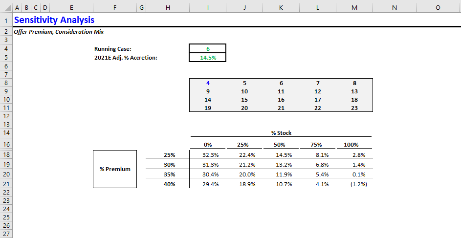
10. Go back to the Sensitivity tab to confirm all cases updated. You should see the following:

Intuitively, this output makes sense. From the acquiror’s perspective, the most expensive offer package is 100% stock with the highest premium (40%).

Offer Premium & Synergies

Okay, we worked through the offer premium and consideration mix sensitivity analysis together. Try to build a similar sensitivity output for offer premium and synergies. You can use the following synergy values:

• 20mm
• 30mm
• 40mm
• 50mm
• 60mm

We’ll use the same offer premium range. Therefore, we’ll need 25 new cases (5 synergy values x 5 offer premium values). Let’s think about how these 25 new cases will differ from the 25 prior cases.

• Offer Premium: We’re sensitizing offer premium in both, so offer premium values should be the same across both sets of cases.
• Consideration Mix: In the first sensitivity (first 25 cases), we showed varying consideration mixes, whereas in the second sensitivity (next 25 cases), we’ll assume 50-50 cash-stock mix throughout. That’s one difference.
• Synergies Furthermore, in the first sensitivity (first 25 cases), we assumed 50mm run-rate synergies, whereas in the second sensitivity, we’re including a range of synergy values (20 - 60mm). That’s the second difference.

Using this information, try to set up the second sensitivity analysis. If you’re stuck, you can always consult the completed version.

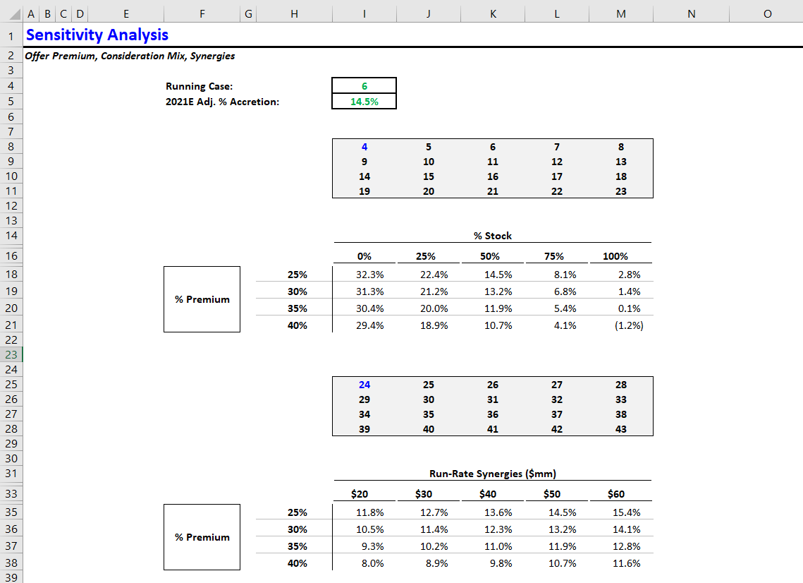
Your updated sensitivity tab (containing both sensitivity tables) should look like this:

Checking Your Work

Bonus points - let’s check those two sensitivity outputs like a VP, who’s not too deep in the weeds.

First, should any of the columns or rows be the same across both tables? (This is called ticking and tying - making sure numbers are consistent across outputs.)

Yes! The first table assumes 50mm run-rate synergies, and the second table assumes 50-50 cash-stock mix. Therefore, the third column (50-50 mix) in the first table should equal the fourth column (50mm synergies) in the second table. We can see that’s the case. So far, so good.

Next, let’s examine each table and verify that the numbers are directionally correct.

We can start with the first table. We know that accretion should decrease when the offer premium is higher (of course, the buyer gets a lower return when they pay more). Therefore, accretion should decrease as we move further down each column. Also, in most cases paying with stock is less accretive than paying with cash. So the leftmost column (0% stock) should have the highest accretion values, and they should decrease as we move right across the table. This checks out.

Now, let’s look at the second table. The same observation regarding offer premium holds: Accretion should decrease as we move further down each column. But unlike the first table, the highest accretion values should be on the right-hand side, because synergies boost accretion. This also checks out.

Conclusion

Now you know the proper way to perform sensitivity analysis. This method is not just for accretion / dilution - it’s for everything. For example, using this approach, you could calculate a sponsor’s IRR under various growth and financing scenarios. It might be intimidating at first, but switching from data tables to self-referencing if statements (+ cases) will speed up your workflow and reduce errors.

Introduction

So far, in our tutorials, we’ve only created single-scenario examples. But when performing financial analysis, that’s unusual - generally you should evaluate a range of potential scenarios and outcomes. The most basic example would be creating a base case, an upside case, and a downside case.

This tutorial is going to build off of our accretion / dilution tutorial. We’re going to show you how to create and test multiple cases, or scenarios. You can apply this approach to any financial model you build.

Rationale

Below are a few reasons to include case functionality in your models.

Inherent uncertainty

When projecting financials, nothing is certain. Will XYZ business unit outperform this year? What will the oil price be? Will shipping costs increase or decrease? You get the idea.

We need to evaluate the financial impact of numerous variables. For example, if shipping costs increase but growth also outpeforms, does that lead to a higher valuation?

Efficiency

Let’s go back to our basic accretion / dilution template (you can download it here). If you want to change a variable (and see how it impacts accretion), you have to overwrite the hard-coded value. Then, if you want to reverse the change, you have to replace the new value. Especially if you’re testing the impact of multiple variables simultaneously, this manual approach becomes inefficient pretty quickly.

Make it explicit

Even if you don’t care about efficiency, it’s still valuable to explicitly define your cases and the variables you’re testing - separate from the main model mechanics. Defining and listing your cases can help you think through what you’re testing. Should I add more variables? Is this too many? Have I defined a downside case?

Teamwork

Furthermore, when you’re working as part of a team, it’s important to define the cases, so that other people can easily open up the model and switch the running case / scenario.

How to add cases to a model

Now let’s add some cases to our basic accretion / dilution template. You can follow along step-by-step, or you can check out the completed version.

Define your variables

The first step is to define your variables - what you’re going to be testing. We’ll be sensitizing / testing the following variables:

• Offer premium
• Consideration mix (% Cash / % Stock)
• Target EPS
• Interest rate on acquisition debt
• Synergies

Build cases tab

Now that we’ve decided on our variables, let’s build out the cases.

1. Create a new tab (we like to call this “MCASE“ - stands for “Main Case” or “Master Case”)

2. Create 1 column per variable - create 1 column for each variable that you’re testing. We’ll create the following columns:

   • Offer Premium (%)

• % Cash
• % Stock
• Target EPS (2020E)
• Target EPS (2021E)
• Target EPS (2022E)
• Acquisition debt interest rate (%)
• Run-Rate Synergies ($mm)

We like this columnar approach, because (among other reasons) it makes it easy to add variables - just add more columns. You don’t have to move your existing cases or alter the other variables.

3. Create label and case column - we like to add 1 column for labels (e.g., “Base Case”) and 1 column for case numbers (1, 2, 3, etc.). These will be the two leftmost columns. Here’s what your column headers should look like:

   

4. Create “Running” row directly beneath the header row(s). This row will display our running case.

• Make the row light gray - this will visually differentiate it from the rows below
• Make the label “Running:”
• Put a box around the case number column (for this row) and center the number. This will be the cell that defines which case is running
• The remaining columns will use the offset function to pull the variables for the specified running case

NOTE: offset might be the most useful function in Excel, so it’s important to fully understand it. The syntax is as follows:

cell value = offset(reference cell, offset rows, offset columns, target rows, target columns)

That might seem like a lot, but it’s actually quite simple. Offset is used to lookup a cell value a specified number of rows and columns away from the reference cell.

• reference cell = where you start from

• offset rows = how many rows to offset. Here, we use the running case number, so if case 1 is running, we move down 1 row; if case 2 is running, we offset 2 rows…
• offset columns = how many columns to offset. Here, we offset 0 columns, because we only want to vary, or offset, the rows. The columns are already lined up
• target rows (always set this = 1)
• target columns (always set this = 1)

Sometimes, it’s easier to see an example and play around with it. Check out the completed version.

5. Create individual cases beneath the running row. You can create whatever cases you want. We’ve created the following:

• Base Case
• Upside Case
• Downside Case
• Offer Premium / Merger Consideration Sensitivity Cases

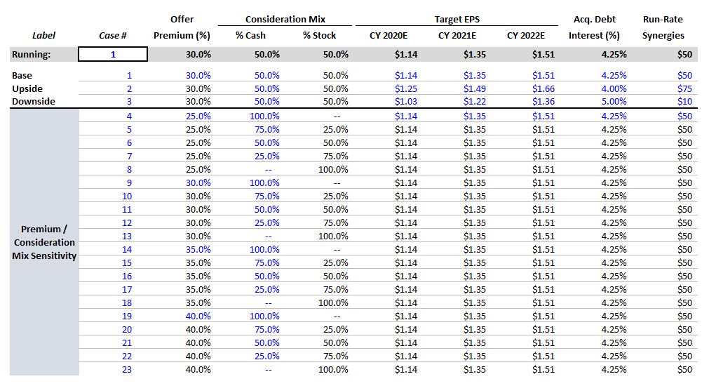
Here’s what our completed cases tab looks like:

Link cases tab to model

Once you’ve built your cases, you can link the running variables back to your model. For example, you can link the target EPS numbers back to the running row on the MCASE tab.

When you change the running case, the entire model updates. Check out the completed version, and let us know if you have any questions.

Introduction

Accretion / dilution was one of the most difficult finance concepts for me to understand when I was starting out. Ironically, it’s one of the simplest. I think the jargon can make it intimidating at first.

This article will introduce the concept of accretion / dilution - how to calulate it and when / why it’s used in financial analysis.

What is accretion / dilution?

Accretion / dilution means:

How much will some per-share financial metric change as a result of a transaction?

That’s it. Generally, it’s used to evaluate the projected change in EPS (Earnings Per Share) resulting from a merger or acquisition. But it’s not exclusive to EPS - the concept can be applied to any per-share financial metric. For example, when evaluating MLP mergers, you might look at the projected accretion / dilution for LP distributions. Why per-share metrics only? We’ll discuss below.

How to calculate accretion / dilution

EPS Accretion / (Dilution) = (Pro Forma EPS - Standalone EPS) / Standalone EPS

Here’s a quick example:

Standalone FY 2020E EPS: 1.00
Pro Forma FY 2020E EPS: 1.25

EPS Accretion / (Dilution) = (1.25 - 1.00) / 1.00
EPS Accretion / (Dilution) = 0.25 / 1.00

So, the proposed transaction is 25% accretive, and we’re projecting a 0.25 increase in FY2020E EPS

Since the PF EPS is greater than the standalone EPS, the deal is accretive. If the PF EPS is lower than the standalone EPS, the deal would be dilutive. Here’s an example:

Standalone FY 2020E EPS: 1.00
Pro Forma FY 2020E EPS: 0.98

EPS Accretion / (Dilution) = (0.98 - 1.00) / 1.00
EPS Accretion / (Dilution) = -0.02 / 1.00

So, the proposed transaction is 2% dilutive

Remember, accretive is positive and dilutive is negative.

Quick Review - Jargon

Finance jargon can be overwhelming at first, but you’ll see the same elements pop up over and over. Here’s a quick review:

• FY 2020E - FY is the abbreviation for fiscal year. A company’s fiscal year can be different from the standard calendar year (1/1 - 12/31). Furthermore, the E after 2020 just means “Estimated” since we’re working with estimated financials for fiscal year 2020.
• Pro Forma - That’s Latin for “as if.” You often see it abbreviated as “PF.” When evaluating a potential transaction, the financial forecasts are Pro Forma, as if the transaction had occurred.

Exploring EPS accretion / dilution

We’ve shown how to calculate EPS accretion / dilution above. Below are some of the factors that influence EPS accretion / dilution in an acquisition:

• Target company earnings
• Synergies
• Cost to realize synergies (synergies aren’t free!)
• Acquisition offer (how much was paid, and what form: cash vs. stock)
• Deal financing (as applicable)

We’ve put together an EPS accretion / dilution template that you can use to explore these concepts and the scenarios below.

All-Stock Deal

This is one of the hypotheticals that always used to trip me up. Ignoring synergies, in an all-stock deal, how do you know if the deal is accretive?

It depends on two factors:

1. Target P/E multiple (using the offer price per share)
2. Acquiror P/E multiple

If company A (20x P/E multiple) purchases company B (10x P/E multiple) in an all-stock transaction, the deal will be accretive. The more expensive stock is buying the less expensive stock.

Here’s another way to think about it:

• 20x P/E multiple means 5% Earnings / Share yield
• 10x P/E multiple means 10% Earnings / Share yield
• If you issue a 5% bond to purchase a 10% bond, the interest income from the 10% bond will more than outweigh the 5% interest expense you owe.
• In this case, company A is the 5% bond (since company A is issuing shares as merger consideration), and company B is the 10% bond (its shares trade at a higher earnings yield).

All-Cash Deal

In an all-cash deal, the acquiror pays the target’s shareholders 100% cash (no stock). The acquiror has to get that cash from somewhere. They have a few options:

1. Excess balance sheet cash (e.g., Apple)
2. Raise debt
3. Raise equity (and pay target’s shareholders with cash proceeds)

For simplicity, we’re going to assume option 2 (Raise debt). In this case, understanding the accretion / dilution is simple: is the acquired earnings yield > the tax-effected interest rate from the acquisition debt?

Here’s an example:

Company A is buying company B for 25.00 per share. Company B has projected EPS of 2.50 and 100 shares. Company A finances the transaction with debt issued at 5%.

Company B has a 10x P/E multiple, or 10% earnings yield.
Company A is issuing debt at 5% pretax (~3.5% post-tax).

The transaction is clearly accretive. Company A will receive extra net income equal to:
162.5 = 25.00 offer price x 100 shares x (10% earnings yield - 3.5% post-tax interest rate)

To calculate the exact accretion we need to know Company A’s share count and EPS. Assuming Company A has 200 shares and projected EPS of 3.00, the deal is quite accretive:

162.5 extra net income / 200 shares = 0.8125 extra EPS
0.8125 / 3.00 = 27% accretive

Mixed Cash & Stock Deals

Use the attached template to explore how the different variables impact accretion / dilution.

Play around with the following assumptions:

• % Premium
• Consideration mix (% Stock / % Cash)
• Interest rate on acquisition debt
• Synergies
• Target & acquiror projected EPS

Why do people care about accretion / dilution?

This is the more complicated part of the story. Let’s start with another question: When evaluating a potential acquisition, what metrics / analyses are most important?

Everything below is a good answer:

1. Valuation of target company / asset (are you paying less than the value you’re receiving?)
2. PF leverage / capital structure
3. PF combined financials / earnings

There are other aspects we’re leaving out that are also important - and that’s partly why evaluating acquisitions is so difficult. A merger or acquisition is a complex problem, and you need to examine it from different angles, which can sometimes tell contradictory stories.

Let’s go back through the list of relevant analyses above.

1. Valuation of target company - this is arguably the hardest piece. Valuation is a notoriously tricky beast with lots of variables and hidden assumptions. Skilled finance professionals can make a DCF tell any story they wish. While other valuation methodologies (e.g., public comparables and precedent transactions) are a bit less numerically subjective, there’s still ample wiggle room: Which public comparables do we select? Which, if any, prior deals are relevant?
2. PF leverage / capital structure - this is the simplest piece. In most cases, leverage / capital structure is a constraint. The financing tail generally does not wag the acquisition dog. Below are a couple examples:

• The acquiror doesn’t want its credit rating downgraded, so it can only raise $Xmm in debt and must fund the rest of the transaction with equity.
• The acquiror’s outstanding debt has covenants that prevent the acquiror from raising additional debt. The acquiror must use equity.

3. PF combined financials - what is the projected financial profile of the company? What synergies is the acquiror predicting, and what is the cost to realize those synergies?

There’s a lot to look at. And that’s one of the main reasons why people like EPS accretion / dilution.

All-in-one Deal Snapshot

Remember: EPS = Net Income / Fully Diluted Shares Outstanding

• Net Income includes the effect of any capital structure change (interest expense), synergies, cost to realize synergies, and the earnings of the acquired company.
• Diluted shares outstanding incude any stock offered as merger consideration.

Thus, EPS accretion / dilution can serve as an all-in-one snapshot of a transaction’s financial impact.

If you believe that:

1. Management’s financial projections (including synergies) are materially accurate and
2. The PF company will trade at the exact same P/E multiple as before

Then, any accretive deal will leave shareholders better off (the stock will trade at a higher price).

Disclaimer

That’s an oversimplification, but it is the basic logic behind EPS accretion / dilution. Let’s examine these assumptions and some of the ways things can go wrong:

• Projected financials - Even when management has the best intentions, projections are always somewhat wrong. The macroeconomic environment can change, a business unit can unexpectedly decline, or maybe the acquiror just does a bad job forecasting the target’s (or their own) financials.
• P/E Multiple - While many stocks trade on P/E multiples, many also trade on EV / EBITDA, or a blend of the two. Some trade based on revenue. And some trade purely on hype. If a company’s stock price trades on EV / EBITDA, then EPS is not as relevant. Likewise, for a material transaction, it’s rare that the trading multiple would remain constant. The market will react; the multiple will change.
• Accretive, but overpay - It’s very possible for one company to acquire another company in an accretive deal, and overpay. EPS accretion is usually a necessary, but never sufficient, condition for a good deal.
• Bad strategy - A company acquires another company for the financial rationale (the deal’s accretive), but the acquisition is a poor strategic bet.

So EPS accretion can serve as a financial snapshot, but you shouldn’t rely on it as your sole guide.

When is accretion / dilution most important?

As you’ve probably gathered, accretion / dilution is most important for public companies. Private companies rarely need to worry about per-share metrics, such as EPS. They often have heavily concentrated ownership and owners who are directly represented on the board of directors.

Public companies face a different set of conditions:

• Diffuse shareholder ownership
• Agency problems (most shareholders not directly represented on the board)
• Public quarterly financial results
• Constant performance measuring stick: company stock price

When undergoing a material merger / acquisition, management teams of public companies face a lot of extra stress navigating these conditions.

• They must communicate to shareholders why the deal is a good use of shareholder capital (vs. returning capital to shareholders & organic initiatives)
• They must sell the public markets on the deal (equity research analysts, major investors, and press)

Even if the management team and the board are convinced a deal is good, they will face severe displeasure if the stock price tanks following a deal announcement. These days, a poorly received acquisition and lackluster earnings are an invitation for activist investors (a.k.a. an extremely persistent migraine).

For these reasons, EPS accretion is often an essential metric for communicating a deal to the public markets. It’s an easy data point that management can refer to in order to show shareholders why a deal makes sense - why it leaves them better off. We’ll make more money for each of your shares, so your shares will be more valuable.

1. Introduction

We’re going to walk through a simple LBO model - it is not meant to be comprehensive. This model (and post) has the following objectives:

1. To teach core concepts and help you develop the understanding required to digest larger models. You can find a more advanced LBO modeling guide here.

2. To help you prepare for paper LBO tests.

Paper LBO
Often in PE interviews, in addition to a full-blown Excel modeling test, interviewers will grill candidates on LBO mechanics in person. You may have to calculate simplified debt paydown and returns calculations by hand. These are called “paper LBOs.”

Here’s an example paper LBO.

Enough philosophizing, let’s get started. Here’s a blank copy of the model, and here’s a completed version with a new tab for each incremental step.

2. Core Assumptions

We tried to keep things as simple as possible, while still giving you a framework for more complex models. Below are the provided assumptions:

Financials

• LTM Adj. EBITDA: $100mm
• Annual EBITDA Growth: 6%
• Annual CapEx: $30mm
• Annual D&A: $25mm
• Annual Increase in NWC: $4mm
• Annual Tax Rate: 30%

Transaction Assumptions

• Cash-free, debt-free: the company is sold with no debt and no excess cash. This is a common assumption.
• Transaction Multiple: 9x
• Transaction Expenses: $30mm

Financing

• Term Loan: 3x Leverage, 4% interest rate, 1% annual amort.
• Senior Notes: 3x Leverage, 8% interest rate

The assumptions under Financials are the bare-minimum required to calculate free cash flow. Under Transaction Assumptions and Financing we have enough information to determine the transaction structure.

3. Transaction

The Sources & Uses section is one of the first steps in every LBO. Quite literally it represents the sources and uses of cash - where is the buyer getting the money from, and what precisely are they using it for?

Let’s start with the Sources.

1. Since we know the leverage multiples for the term loan and the senior notes, we can calculate the debt raised for each tranche by multiplying the respective leverage multiple by LTM Adj. EBITDA.
2. We’ll come back to the sponsor equity. We’re going to use it as the plug to bridge the gap between total funds required and debt financing.

Uses
How do we get the equity purchase price? We have the LTM Adj. EBITDA and the Transaction Multiple, so we can calculate the Enterprise Value (a.k.a. the Transaction Value).

Transaction Value = LTM EBITDA x Transaction Multiple

We also know the relationship between Enterprise Value and Equity Value:

Enterprise Value = Equity Value + Net Debt

But remember: the transaction is cash-free, debt-free (net debt is $0), so the equity value equals enterprise value. Therefore, our Purchase Equity = LTM Adj. EBITDA x Transaction Multiple.

The transaction expenses are an illustrative assumption, so now we have total uses of cash.

Let’s go back to the Sources. We’ll set Sponsor Equity equal to the Total Uses - Debt. This mirrors actual deal dynamics - sponsors generally try to raise as much debt as possible. They pay for the rest.

Sponsor Equity = Total Uses - Term Loan - Senior Notes

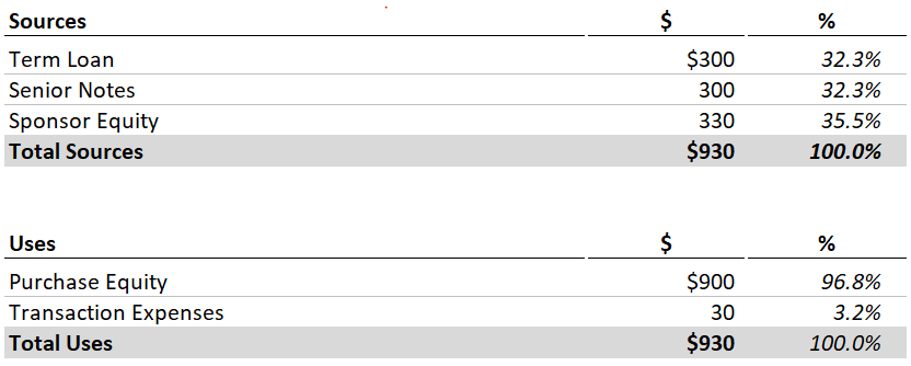
Your Sources and Uses should look like this - check the completed model if you’re having trouble.

4. Cash Flows

Most of these line items should be familiar. Try to fill out as much as you can using the provided assumptions. You’re missing interest expense, so you can leave that out for now.

Your completed Cash Flows schedule should look like this:

You may be wondering: Where’s revenue? Good question. Since we’re making up numbers, no need to show revenue. EBITDA feeds into Net Income and, ultimately, Levered Free Cash Flow.

Here, using detailed financials is unimportant. For private equity investors, the opposite is true. Diligencing a company’s cash flows and building a detailed operating model are among the most important parts of the investment process.

For now, let’s stick to the financial mechanics.

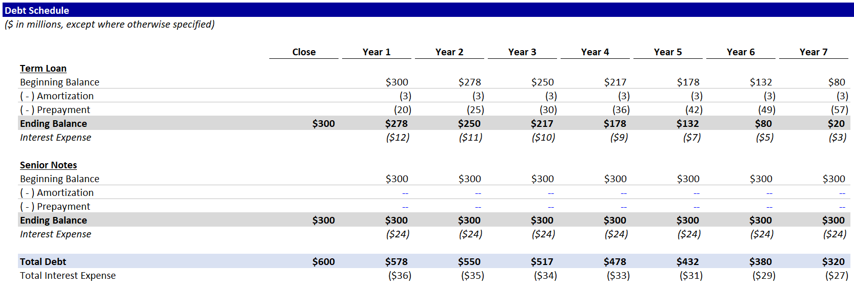
5. Debt Schedule

Term Loan

1. Set the ending balance in the Closing column equal to the amount calculated in the Sources & Uses. This represents the amount outstanding immediately after the transaction closes.
2. Set the beginning balance in Year 1 equal to the ending balance at close.
3. Set the ending balance in Year 2 equal to the sum of the beginning balance, amortization and prepayment. Since amortization and prepayment are blank, the ending balance should equal the beginning balance. Copy these formulas across.

   Ending Balance = Beginning Balance - Amortization - Prepayment.

4. Go back to our assumptions. We know that the Term Loan has annual amortization of 1%. This means that the company must pay 1% of the initial loan amount to the lenders each year. Try to fill out the correct formula, but be careful - loan amortization is a percentage of the initial amount, not the beginning balance each year.

Term Loans
Term Loans are a common source of debt financing for LBO transactions. To learn more, you can check out LeveragedLoan.com. Our more advanced LBO guide includes additional resources.
5. Onto Prepayment. For illustrative purposes, let’s set prepayment equal to available cash flow each year. This is a big simplification. Ordinarily, each debt tranche would have specific rules about when and how much they can be paid back early. Why would they want to limit being paid back early? If there weren’t limits to prepayment, companies could refinance outstanding debt whenever rates decreased, and they could leave debt in place whenever rates increased. Debt investors would be hosed. The reality is that companies do this anyways, but they have to pay debt investors extra fees for prepayment, and sometimes the fees can be quite onerous. Of course, the terms of prepayment and associated fees vary greatly by type of debt and specific issuance.
Cash Available for Prepayment = Levered Free Cash Flow - Mandatory Amortization
6. As a simplification, let’s calculate interest expense using the Beginning Balance each year. Ordinarily, we would use an average of the beginning and ending balances to account for the fact that debt is being repaid over the course of the year. This leads to Excel’s dreaded circular reference, as the more advanced guide explains. Let’s keep things simple.
Interest Expense = Beginning Balance x Interest Rate

Senior Notes
Now, it’s your turn. Replicate these calculations for the Senior Notes with a couple key differences:

1. Amortization is 0 in every year (you can hardcode it).
2. Prepayment is also 0.

   Senior Notes are one of the types of debt that usually have steep penalties for prepayment. Furthermore, the term loan is senior to the notes in the company’s capital structure, which is a fancy way of saying the term loan must be paid back first.

Total Debt

1. Calculate total debt in each year as the sum of the ending balances.
2. Sum the total interest expense and link it back to the Cash Flows schedule.

Other Comments
We’re not calculating a cash balance anywhere, because all excess cash flow goes to paying down the Term Loan.

Your completed Debt Schedule should look like this:

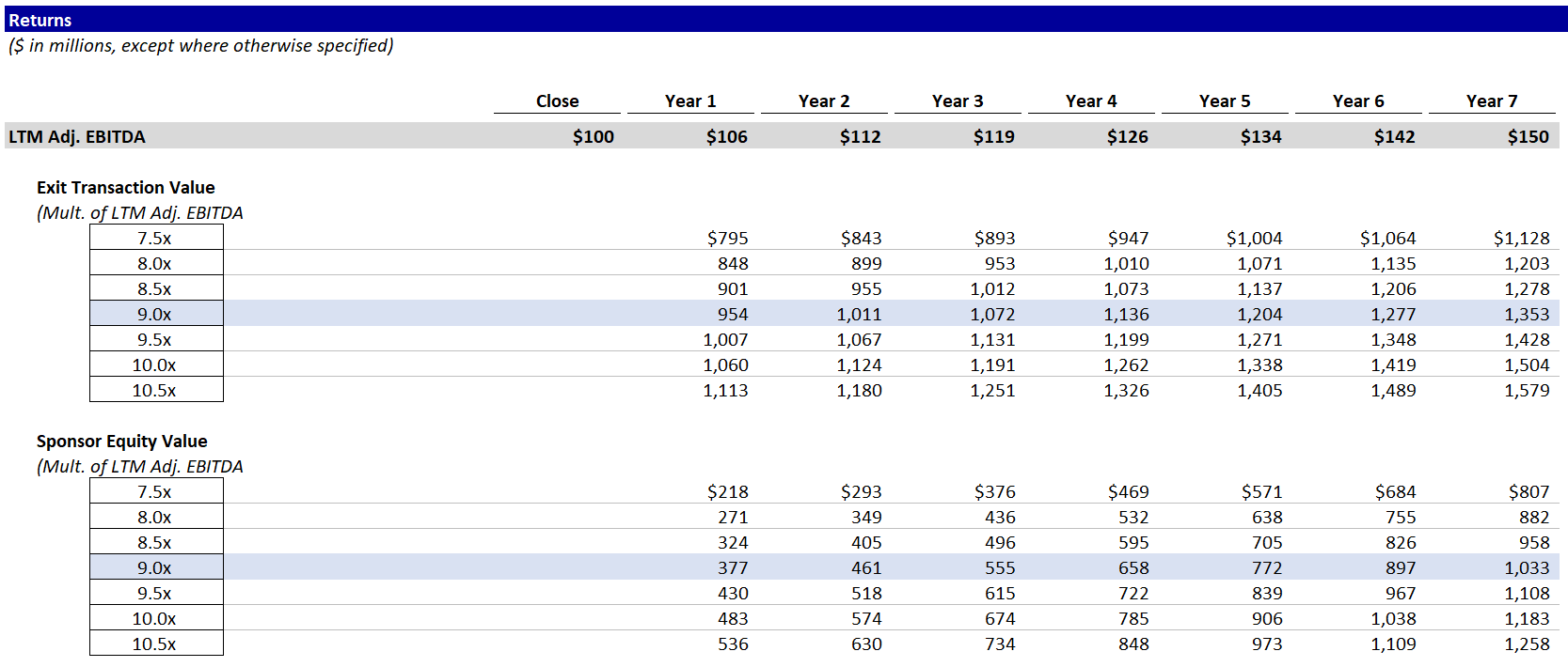
6. Returns

Now let’s find out how much money this sponsor is going to make.

1. Link LTM Adj. EBITDA from the Cash Flows schedule.
2. Calculate the Transaction Value at exit for each year at each multiple.

   We’re showing a range of multiples, because the sponsor never knows how much they’ll sell the business for. This allows us to answer questions like - if we exit in 5 years at 7.5x, what do returns look like?

3. Calculate the future equity value using the range of transaction values from the step above. We’re not building a cash balance, so Net Debt = Total Debt.

   Equity Value = Transaction Value - Net Debt

4. Next up - MoIC: Multiple of Invested Capital. That’s PE speak for “how many times our money will we make?”

   MoIC = Equity Value at Exit / Invested Equity

5. For simple transactions like this LBO (one cash inflow and only one outflow), we can derive the IRR from the MoIC:

   IRR = MoIC ^ (1 / year) - 1

IRR and MoIC are the 2 most common metrics for evaluating PE transactions. And they’re better together. MoIC makes it easy to understand the profit from a transaction, but it does not take into account the time value of money. IRR does factor in time.

Your completed returns schedule should match this:

7. Next Steps

Congrats on completing the Easy LBO! Try the rest of our private equity modeling tutorials:

1. Intermediate LBO Guide
2. Advanced LBO Guide
3. Ability-To-Pay Analysis
4. LBO Value Creation
5. Private Equity Modeling Guide

Introduction

If you have not read Tax Principles (part 1) yet, please start there.

–

Now that you have a basic legal / tax model for corporate entities, let’s begin looking at specific tax assets. We’ll start with Net Operating Losses, commonly referred to as NOLs. NOLs are exactly what they sound like - losses accrued over time.

Why are NOLs valuable? Because subject to certain restrictions, corporations can use NOLs to shield taxable income, i.e., avoid paying taxes. Going back to our first principles, the US goverment wants a piece of every dollar of profit. Corporations and corporate profits, however, are not one-and-done transactions. Companies often make investments that span multiple years, and then reap the profits over ensuing years and possibly decades.

Example: consider a startup consumer products company that must invest heavily in its brand in the early years. It may incur losses for several years, before sales catch up to advertising expenses. The company would have no taxable income in the early years (losing money every year), and then it would be hit with a full tax bill once the business starts to turn around.

Instead, NOLs provide a mechanism to balance out profits and losses over the years. A company that loses money in one year can carry over those losses to offset future profits.

Basic Rules

1. NOLs can be carried back to the preceding 2 tax years and applied for an immediate tax rebate; or they can be carried forward for the next 20 years.
2. After 20 years, any remaining NOL balance is canceled.
3. Going back to our first principles, tax assets are depletable resources, so NOLs can only be used once.

Valuing a Standalone Company’s NOLs

You can value NOLs using a simple DCF. Like any other DCF, the key inputs are the cash flows and the discount rate.

Determining the Cash Flows

Let’s start with the cash flows. Assuming you’re valuing a company’s existing NOL balance (no new NOLs are created), the balance is a wasting asset. It grows smaller with use and eventually will be fully exhausted or canceled. The annual use of NOLs are a function of the company’s profitability. If the company is projected to be highly profitable, it will be able to use the NOL balance more quickly, and vice versa. To calculate the annual cash flow, the formula is simple:

Annual cash value of NOL = taxes shielded = NOL balance used x Tax Rate

Obviously, the value of the NOLs increases if the company is able to use them more quickly (time value of money).

What discount rate should we use?

That is subject to disagreement, duh. Many finance professionals like to use artificially low discount rates, because they argue that the risk is quite low (not comparable to equity risk). This has the fortunate effect of making the calculated asset value higher than it would be if one were to use a higher discount rate.

While a low rate may be appropriate in select cases, I think a more appropriate discount rate is somewhere between the company’s cost of debt and its cost of equity. Look at the order of payments in the income statement. First comes interest expense, then taxes, and last net income. Interest expense is a pretax item. Therefore, debtholders are paid before the government, and tax payments can be considered riskier than debt payments. The government, however, is paid before net income and shareholders. Therefore, the discount rate should reflect the relative risk - it should be between the cost of debt and the cost of equity.

Sample DCF Output

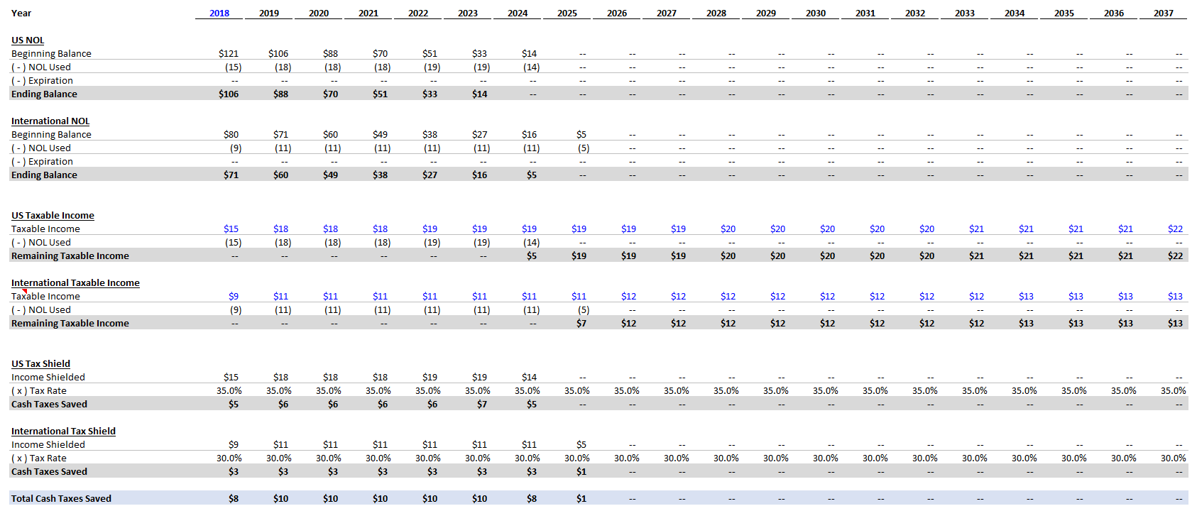
Below is a sample DCF output, showing the build to cash taxes saved. Here is the full excel file (containing this output and the rest of the outputs from this article).

Standalone NOL Valuation Gotchas

1. Do not double-count the value of the NOLs by valuing them separately if they’re already baked into the company’s projected cash taxes paid. Rule of thumb: if you’re valuing the NOLs separately, do not include them in your main corporate DCF.
2. If you value the NOLs separately, the timing of projected tax shields (via NOL) must be consistent with the company’s projected income.
3. If you are going to the trouble of valuing a company’s tax assets, you should pay attention to jurisdiction. In public filings, especially if the NOLs are material, companies often disclose a breakdown by jurisdiction. You can also usually get the company’s approximate operating income in those jurisdictions. NOLs should only be used to offset income in the matching jurisdiction.
4. Tying into the item above, different tax jurisdictions have different rules. The approach discussed in this article is US-centric. Not all jurisdictions are the same. Do some googling.

Valuing an Acquisition Target’s NOLs

As you might imagine, tax assets make tasty snacks. Unfortunately, the IRS wants to limit the trafficking of NOLs - cases where corporate shells are purchased solely for the residual tax assets. Enter Section 382 of the Internal Revenue Code (IRC).

Section 382
I’m only mentioning the IRC section here so that if someone references it, you’re not lost. The important part is understanding the rule, which is simple: acquired NOLs are subject to a maximum annual use constraint, which is referred to as the Section 382 Limitation.

Section 382 Limitation = Fair Market Value of AcquiredCo x “Federal Long-Term Tax-Exempt Rate”

The Federal Long-Term Tax-Exempt Rate is one of several rates that the IRS publishes periodically and is used in many similar tax calculations. You can find the latest rate on the IRS website. Generally though, if you google “Federal Long Term Tax Exempt Rate,” you can find it pretty quickly.

For financial modeling purposes, you can assume the FMV of AcquiredCo equals the calculated equity value in your acquisition analysis (enterprise value - net debt). The tax definition of the FMV can be more complicated, and there are nuanced games that can be played to manipulate the value. The acquiror wants the FMV to be deemed as high as possible for tax purposes, so that they can use more of the acquired NOLs, more quickly.

Below is an example valuation analysis of an acquired company’s US NOL balance. Here is the Excel file if you didn’t already download it.

Introduction

Taxes are an important consideration in most transactions, especially for deal structuring. Unfortunately, many finance professionals (bankers and PE investors) are unnecessarily intimidated by the subject. While the legal minutiae are best left to the experts, understanding core tax concepts and being able to think (and speak) intelligently about tax structuring are within every deal professional’s grasp.

This article will be the first in a series of articles exploring important tax concepts for finance professionals, including (in no particular order):

• asset acquisitions vs. stock acquisitions
• valuing tax assets (e.g., NOLs)
• tax-free transactions

Before we get to the fun stuff, however, we need to review some core concepts. These will build the foundation for thinking about tax structuring and researching problems that you haven’t encountered before.

First Principles

1. The US government wants a piece of every dollar of profit.
2. In order to make calculating profit straightforward, the government usually waits until the profit has been realized, i.e., a transaction has occurred.
3. Deductions, or other forms of tax shields, are a depletable resource. They can only be used once.

Basis, Basis Everywhere

The concept of basis is critical to understanding tax – and deal structuring. Basis is the amount you invested in acquiring an asset. It’s how much you paid for it. Going back to the first principles above, you need to know how much something cost in order to determine your profit, which the government will take a piece of.

Simple Example: Buying Stock

• Year 1: You pay $10 per share for 10 shares ($100 aggregate basis).
• Year 2: The shares are worth $20 per share. You still have an aggregate basis of $100, and you have an unrealized gain of $100.
• Year 3: You sell half your shares for $250. Half of your basis is $50. Therefore, you have a profit of $200 ($250 - $50), which you pay taxes on. Your basis in the remaining shares is $50.

First Principles: You pay taxes when your profit is realized. Your basis is how much you invested.

Next, let’s check out a slightly more complex example.

More Complex Example: Depreciation

• Year 1: Company A buys a factory for $100. Basis is $100.
• Year 2: Company A deducts $20 of depreciation from taxable income (depreciation is tax-deductible). Basis is $80.
• Year 3: Company A deducts $20 of depreciation from taxable income. Basis is $60.
• End of Year 3: Company A sells the factory for $80. It realizes a taxable profit of $20 ($80 of gross proceeds - $60 basis).

First Principles: You pay taxes when your profit is realized. Basis is how much you invested, but a given tax shield may only be used once. Since Company A deducted depreciation, when the company sold the factory, it had a lower basis, and the company faced a larger taxable gain.

P.S. If you wish to go deeper down the rabbit hole, research tax depreciation, a tricky subject that is even trickier to model. Tax depreciation does not conform to GAAP or IFRS depreciation formulas. The IRS has its own nuanced rules, which you can read about here. The depreciation rates (MACRS) can be found starting on page 71.

The Corporate Shell (a.k.a. the marble bag)

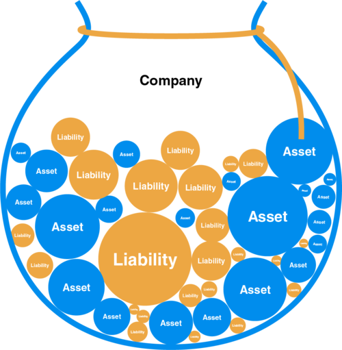
Now that you understand the concept of basis, let’s establish a new model for thinking about companies (from a legal / tax perspective): the corporate shell. Companies are really shells, which own/contain a collection of assets and liabilities. Companies have basis in each owned asset – even if that basis is quite low (many companies have depreciated some of their assets to a basis of $0). The image below is a good illustration of the corporate shell (a.k.a. the marble bag).

Companies can come in a variety of legal forms (partnerships, LLCs, corporations, etc.). We won’t cover the (dis)advantages of these variations here - you can find many good overviews elsewhere. For example:

• Benefits and Drawbacks of Different Types of Business Entities
• Shorter Overview

The important part is reframing your mental model of companies. If you’re like me, you may have started out thinking of companies as amorphous blobs, but it’s better to picture them as shells containing a collection of individual assets and liabilties. Shareholders have basis in their shares, and companies have basis in their assets.

To be continued…

Introduction

Ah, the dividend recap. It’s one of those phrases attached to private equity that gets tossed around without much explanation. You’ve probably heard the phrase, maybe read a DealBook article, but never worked on one. You may have some questions:

1. What is a dividend recap?
2. When and why would a financial sponsor pursue a dividend recap transaction?
3. How should we model a dividend recap?

This article will strive to answer these questions in order.

1. What is a dividend recap?

‘Dividend recap’ is short for ‘Dividend Recapitalization,’ so it’s a recapitalization transaction + a dividend.

Great, what’s a recapitalization transaction? A recapitalization is when a company’s capital structure (the mix of debt and equity and other sources of capital) is adjusted.

Financial sponsors use dividend recaps as one of their many tricks to boost returns. Typically, sponsor-backed companies have a sizable debt load, and all excess cash flow is used to pay down debt. A dividend recap enables the sponsor to pay themselves a dividend before paying down the debt.

Wouldn’t debt covenants prevent that? They would. That’s where the recapitalization piece comes into play. In order to free the company from the restrictive debt currently in place, the sponsor refinances some or all of the company’s outstanding debt. The new debt is used to (a) repay the old debt and (b) finance a dividend to the sponsor.

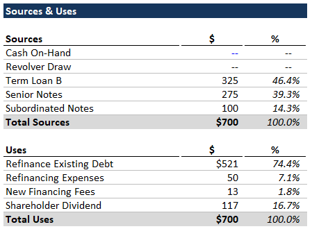
Below is an illustrative sources & uses for a dividend recap transaction:

Note the refinancing costs - these can be quite expensive depending on the type of debt that the sponsor-backed company has in place. Some types of debt include a penalty for early repayment, and generally speaking, bonds are much more punitive than bank debt.

2. When and why would a financial sponsor pursue a dividend recap?

A number of criteria must align for dividend recaps to make sense - these are outlined below:

1. The company has capacity for (significantly) more debt. When the company raises new debt, it must first pay back the existing debt, along with fees, and then whatever’s left over can be paid out as a dividend. If the company cannot raise meaningfully more debt, why bother?

2. Credit markets are favorable and willing. In tightening credit markets, investors don’t look favorably upon this type of transaction. In bouyant markets, (1) debt investors tolerate more leverage, and (2) cheaper interest expense means a company can service a bigger debt load (all else equal).

3. Credit markets have improved since the company’s original debt issuance. This is a nice-to-have. Improved credit conditions make dividend recaps more favorable (they make the math work better), because there is more value in the refinancing piece of the transaction. A company may save money by replacing expensive debt (higher interest expense) with cheaper debt.

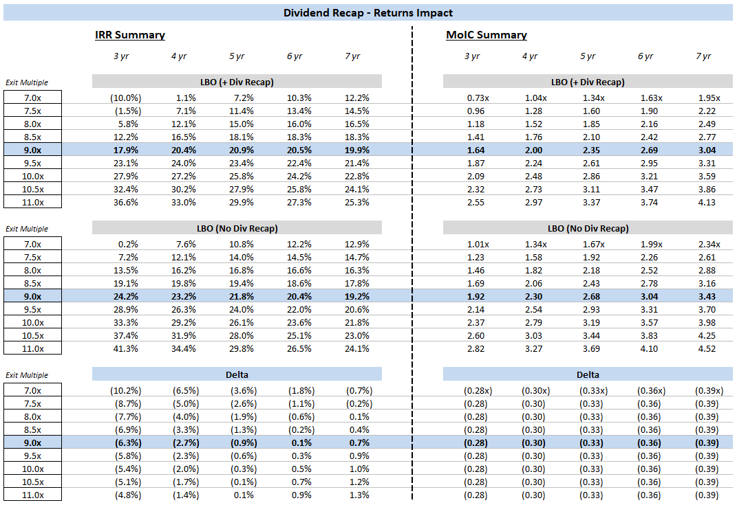
Below is a comparison of sponsor returns - with and without a dividend recap. We’re assuming $50mm in refinancing costs and the same financing terms as the original LBO. As you can see, given those assumptions, a dividend recap is not helping returns. You can play around with the assumptions and see the returns impact. Model attached.

Other Considerations

1. Taking money off the table. While dividend recaps generally increase a company’s financial leverage, they may decrease the total investment risk, because they allow the sponsor to immediately recoup some of their initial investment. There have been a number of cases in which sponsors recouped their entire investment via dividend recap and then later sold the company for extra $$$.

2. Fundraising Optics. If a sponsor is in the midst of fundraising, dividend recaps can help weave a story of “high-performing recent investments.” The total outcome is unknown until the sponsor exits, but a dividend recap can help signal that things are going well.

3. Sponsor can’t find an attractive exit and wants to buy some time. This one is pretty self-explanatory.

3. How should we model a dividend recap?

First, what is our modeling objective?

1. We want to add dividend recap functionality to an existing LBO model.
2. We want to be able to toggle it on and off.
3. We want to be able to choose the year in which we perform the dividend recap.

Next, some simplifying assumptions:

1. If we perform a dividend recap, we refinance all existing debt.
2. Same credit terms and structure as the original debt issuance, but you are free to adjust.
3. For the selected year, the dividend recap occurs at the very end of the year.

Like any modeling exercise, we need to break this into pieces. There’s the dividend and the recapitalization. The dividend is easy to model - a reduction in shareholder’s equity and a few adjustments to the investor returns calculations.

The recapitalization is more complicated. We need to dynamically calculate debt capacity and sources & uses based on the LTM EBITDA for the selected year. Then, we need to add the refinancing and new debt line items to the debt and interest expense schedules.

Download the following files:

• LBO Model (no Div Recap) - base LBO model, which we’ll use to build the dividend recap functionality.
• Completed Model (w/ Div Recap) - for your reference. This Excel file includes a tab for each step of the tutorial.

If the LBO looks overwhelming, pause and work through our LBO modeling tutorial.

The steps/instructions below are meant to accompany the completed Excel file.

Step 1. Build out new Sources & Uses and transaction assumptions.

1. Add Dividend Recap controls to the main Transaction Assumptions section. Remember - we want to be able to (a) toggle the dividend recap on and off and (b) pick the year.
2. Create a new Dividend Recap Transaction Summary section beneath the Transaction Assumptions section. Just like the debt financing for the main LBO transaction, all debt raised will be based on the LTM Adj. EBITDA - but for which year? This is where it gets tricky.
3. The first piece of the Dividend Recap Transaction Summary should be a Key Metrics section where we specify the LTM Adj. EBITDA and the total debt to be refinanced. See if you can come up with a formula for the correct EBITDA using the Excel offset() function and the assumed year of the dividend recap.
4. Next calculate the debt raised (based on leverage multiples) and associated financing fees.
5. Fill out the Sources and Uses. Assume $50mm of debt refinancing costs (purely illustrative). In real life, you’d be able to calculate the exact fee based on the bond indentures or other debt agreements.

Step 2. Add new debt line items to the Debt Schedule.

Now we need to expand the Debt Schedule to accomodate the new debt tranches. Under Ending Debt Balance, Mandatory Amortization Schedule, Mandatory Amortization, and Optional Prepayment, create new rows for the debt raised under the dividend recap. The one exception is the revolver. No need to replicate that – we assume it is refinanced at exactly the same terms as the original issuance.

Be careful with the total formulas for each section. Also, the starting debt balances for the dividend recap tranches can be set to 0 for now.

Step 3. Add new debt line items to the Interest Expense Schedule & update Credit Metrics.

1. Similarly, add rows for the new debt tranches and be careful with sum formulas.
2. For amortization of deferred financing fees, you can link the total fees to the Dividend Recap Sources & Uses, but the amortization should be 0 if the transaction is toggled off, or if the given year is before the year of the recap.
3. Likewise, be careful with the formula for PIK interest expense. Consult the completed file.
4. Update the Credit Metrics. Change the formulas for the Senior Secured Debt, Senior Debt & Total Debt rows to include the new debt tranches.

Step 4. Build Adjusting Line Items Schedule.

Next we need to integrate the dividend recap with the rest of the model. The debt schedule functions, but all of the new debt tranches should be 0, since we haven’t dynamically linked the starting balances.

1. Create a new section underneath the Dividend Recap Transaction Summary, entitled Dividend Recap Adjusting Line Items. Here we’re going to create an adjustment row for each item affected by the transaction. If we need a reminder on which line items these should be, let’s look at the Sources & Uses:

   • existing debt tranches refinanced
   • new debt tranches added
   • refinancing costs and dividend reduce shareholders’ equity
   • new financing fees capitalized in other noncurrent assets

2. When calculating the debt to be refinanced, you basically need to duplicate the calculations under Ending Debt Balance in the Debt Schedule, because we’re going to subtract this (calculated) amount in the Ending Debt Balance section. If we just linked to the Ending Debt Balance, we’d have a nasty circularity.

Term Loan Ending Balance = Beginning Balance - Mandatory Amortization - Optional Prepayment

Notes Ending Balance = Beginning Balance - Mandatory Amortization - Optional Prepayment + PIK

Once you have the debt to be refinanced, add it back to the Dividend Recap Sources & Uses. The rest of the calculations should be relatively straightforward.

Step 5. Incorporate adjusting line items.

Now we need to incorporate the adjusting line items in the rest of the model.

1. Add debt refinancing and new debt tranches.

We need to add the debt refinancing and the new debt tranches to the Debt Schedule. In the Ending Debt Balance calculation for the original LBO debt tranches, subtract the refinanced debt (which should equal the sum of other items). Therefore, if the dividend recap is toggled, the Ending Debt Balance for these tranches should be 0 in the year of the recap.

For the new tranches, do the opposite. Add the amount of issued debt to the Ending Debt Balance calculation.

Now you should see a distinct pattern in the Ending Debt Balance section. In the year of the recap, the LBO tranches are set to 0, and the recap tranches appear. The recap tranches delever thereafter.

The interest expense schedule should update automatically, but scan through it. It’s an easy way to catch any sloppy sum formulas.

2. Balance Sheet Adjustments

Add capitalized financing fees to Other Noncurrent Assets.

Subtract refinancing costs and the dividend from Shareholders’ Equity.

Step 6. Adjust returns calculations.

I’ll summarize, and you can try to implement these changes yourself, and then reference our completed version.

1. The dividend amount needs to be added to the numerator in MoIC calculations for all years after (and including) the year of the dividend recap.
2. IRR - you need to add a separate cash flow schedule (with a corresponding IRR calculation) for each exit year. Since the sponsor is receiving cash flows in multiple periods (they get the dividend one year and sale proceeds another year), the typical IRR formula (using MoIC) no longer works.

Use the XIRR() function for the IRR calculations, and you can combine the results for each exit period in a single table - mirroring the format we had prior to the dividend recap.

Next Steps

If you really want to see the returns impact, you should examine multiple sets of financing assumptions. Rig up a few financing cases for the dividend recap (improved case, worse case) and vary those along with the refinancing costs.

Try the rest of our private equity modeling tutorials:

1. Easy LBO
2. Intermediate LBO Guide
3. Advanced LBO Guide
4. Ability-To-Pay Analysis
5. LBO Value Creation
6. Private Equity Modeling Guide