Standalone Model (Part 2) - Parsing the Historical Data

Introduction

This is the second post in our tutorial series showing you how to build a detailed standalone model for Slack Technologies, Inc. (NYSE: WORK).

In our prior article, we introduced public filings research and showed you how to calculate enterprise value and implied trading multiples. Together, we built a Public Market Overview (PMO) for Slack.

Now, we’re going to explain the art of parsing a public company’s filings in order to model the company’s future performance. Each company’s financials form a unique puzzle, and deciding which line items to focus on requires significant judgment. Furthermore, many companies’ disclosures are inconsistent over time (as we will see with Slack).

This article will guide you through Slack’s historical financials. We will show you how to weigh which data points to include, and which to ignore. We will also detail the process for collecting cleaned quarterly data, which will be the input for our next article on building operating cases. A model without clean data is an exercise in futility.

High-Level Discussion

It’s natural to start a modeling project by diving into financial statements and entering numbers in Excel. I’m guilty of that myself. Guilty!? Isn’t that what you’re supposed to do? Well, yes, but let’s take a minute to map things out and discuss what we’re looking for first.

If you think about it, financial statements are actually an output. We read them and perform analyses in order to draw inferences from the data. Does the given company have strong cash flow? How are its unit economics trending? We take the financial statements, the output, and we try to better understand the machine that produced them, the company.

Financial modeling, when done right, should normalize this order of operations. We model the drivers of the business, and the resulting financial statements are once again an output. So how do we find and model the key drivers for a business?

Building an Operating Model

That question is the crux of building an operating model. The first step is familiarizing yourself, at a high-level, with the given company and its business model.

If you’re unfamiliar with a public company, or its business model, skimming its latest 10-K is a great place to start. Here’s Slack’s latest 10-K.

Once you know the basics, the next step is identifying the key metrics for that business model. What information / line items would you need in order to make an illustrative income statement? You definitely need to know revenue drivers, preferably unit prices and volumes. Likewise, you need to understand the cost structure, CapEx requirements, and working capital.

Applying this framework to Slack, let’s start by identifying Slack’s business model. Slack is a Software-as-a-Service (SaaS) company. SaaS businesses make money by charging customers monthly, quarterly, annual, or multi-year subscriptions. You can break down a SaaS business’ revenue model into several variables:

  • Number of customers
  • Average subscription ($) per customer
  • Average churn (percentage of customers that leave over a given time period, e.g., monthly churn)
  • Number of projected new customers

Ideally, you’d have this historical data by customer segment (the specific customer segments depend on the business) or cohort (dare to dream). But you’re unlikely to find this data for a public company, even in aggregate. You have to make do with what’s available.

On the cost side, SaaS businesses are straightforward:

  • Sales costs are a variable expense, since reps get paid commission for new deals and renewals.
  • Customer support should be a variable expense (tied to number of customers or revenue).
  • Computing infrastructure costs (e.g., AWS) should be relatively fixed / a step function.
  • You can think of R&D (product & engineering) as a mix of growth and maintenance CapEx. Most SaaS businesses invest heavily in product, especially in the early years. To be conservative, we can model R&D as a variable cost.
  • Marketing is also a variable expense, but it’s a weird one, because marketing dollars spent today will earn money far into the future (hello, subscription revenue). Marketing expenses should be connected to customer growth (more marketing dollars = more new deals).
  • Lastly, G&A is somewhat of a step function, but can be modeled conservatively as a variable cost.

Just like on the revenue side, we’ll have to make do with what’s available. We won’t get everything. But now you should have a clearer understanding of the operating drivers we’re looking for.

Fixed vs. Variable Costs
You probably already know the distinction, but it’s worth covering just in case. Fixed costs are costs that do not change as a function of sales in the near-term. For example, you probably won’t get a new office if you sell 5 more units tomorrow. The office rent expense is a fixed cost.

Variable expenses, well, vary with revenue. For example, you sell pencils. If you sell more pencils, you will spend more money on wood and graphite (inputs) and labor (to make pencils). These are variable costs.

Summary

So far, we’ve:

  • Identified Slack’s business model, Software-as-a-Service (SaaS).
  • Discussed key revenue and cost drivers.

Now, we’re going to:

  • Comb through Slack’s financials to assess what data is available.
  • Pull and clean Slack’s historical data.

Assessing What Data’s Available

We’ve discussed the metrics on our wish list. Now, we need to assess what’s actually available. To that end, I recommend the following:

  1. Read the latest 10-Q.
  2. Skim the latest 10-K. Here the focus is on surveying what’s included rather than reading the content.
  3. Read the latest earnings release. This is the Exhibit 99.1 that’s included as part of the 8-K immediately preceding a 10-Q/10-K. (If a company releases multiple 8-Ks on the same day, you may need to click on several to find the earnings release.) The earnings release is usually where management discloses non-GAAP metrics.
  4. Check the prior earnings release to confirm it’s consistent with the latest one (sometimes companies are inconsistent).

The good and the bad news is that Slack doesn’t provide much besides the mandatory disclosures. That’s good, because it means less work, and it’s bad, because it means we have less operating data for building projections.

Price / Volume Data

In the latest earnings release, Slack provides the following data points:

  • Number of customers (total)
  • Number of customers paying $100,000+ annually
  • Number of customers paying $1,000,000+ annually

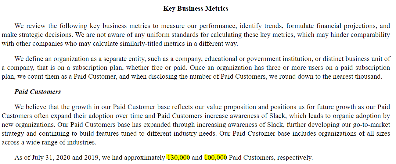
Likewise, in the 10-Q, Slack offers a couple additional nuggets. First, under Management’s Discussion and Analysis (MD&A), there’s a section titled “Key Business Metrics,” which reiterates the customer counts.
Customer Pricing

More importantly, the Key Business Metrics section of the 10-Q includes the percentage of revenue allocated to customers paying $100,000+. Therefore, we also know the percentage of revenue contributed by all other customers (those paying less than $100,000 annually).

This data point is crucial, because the customer counts alone do not enable us to create a detailed revenue build. Now that we have the percentage of revenue by customer segment, however, we can calculate the revenue per segment (segment percentage x total revenue). Then we can divide the revenue per segment by the segment customer count in order to derive the average revenue per customer. This is essentially the unit price, so we have price / volume data by segment for a detailed revenue build.

Since Slack doesn’t disclose the percentage of revenue from $1,000,000+ customers, we’ll ignore them. Instead, we’ll focus on two segments: large customers ($100,000+) and everyone else. Anyways, $1,000,000+ customers are implicitly bundled as part of the $100,000+ segment.

Quick aside - it’s fascinating seeing how much of Slack’s revenue (~50%) comes from its biggest customers. This is a key diligence area:

  • Can Slack continue converting smaller customers into big customers?
  • How well does Slack retain its largest customers?
  • Has Slack lost any big customers?
  • What do Slack’s largest customers have to say about the product?

Free Users

In addition to customer counts, the prior earnings release also includes the total number of organizations using Slack (free and paying). Since we know the number of customers, we can deduce the number of free organizations, which is important, because Slack has a freemium sales model. Organizations can begin using the product, and proving value, for free. At a certain point, they reach a paywall and must convert to paying customers. Therefore, the pool of free organizations forms Slack’s supply of potential customers.

When projecting Slack’s revenue, we’ll need to think carefully about the number of free organizations using Slack and what percentage we expect to ultimately convert to paying customers.

Customer Retention / Churn

You may have noticed that Slack also discloses a Net Dollar Retention Rate.
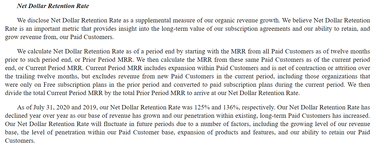
It took us a few reads to understand what this metric represents. Basically, for any period, Slack looks at its customers a year prior and compares the revenue from that group a year ago to the revenue from that group today. This metric ignores new customers (won in the past year) in order to measure the aggregate impact of:

  • Churned customers
  • Existing contract increases
  • Existing contract decreases

Ideally, we would like to include this metric as part of our revenue build, but unfortunately, it combines too many separate variables. We also have no knowledge of its breakdown by customer segment. Therefore, we’re not going to focus on net dollar retention when building our operating model, but it is a metric an investor would want to watch.

Cost Data

On the cost side, Slack’s disclosures are pretty light. Hosting costs are the one detail we can glean from the 10-Q notes:

As we discussed above, hosting costs are relatively fixed, but follow a step function. The contract minimums should serve as a good proxy for future costs. Also, in the income statement, hosting costs are contained almost entirely within the cost of revenue line. This enables us to disaggregate hosting costs from the cost of revenue, and we’ll assume the remaining cost of revenue consists of variable support costs.

The 10-Q notes also contain office lease commitments. But unfortunately, rent expense is allocated among several income statement line items. Therefore, it’s impossible to disaggregate, and doing so would add little value.

We’ll pull all other cost data from the income statement.

CapEx and Working Capital

Likewise, we’ll find CapEx in the statement of cash flows, and we’ll pull working capital directly from the balance sheet.

1) Starting in Excel

Enough chitchat - let’s start pulling & cleaning some data.

We’re going to start with the final Excel file from our prior article.

And here’s our updated Excel file containing Slack’s cleaned historical financials and operating data. Even if you don’t want to go through this exercise manually, we recommend you skim the guide / discussion below.

Note on Data Scrubbing
Personally, I find pulling and cleaning data extremely tedious, but going through the process always unearths some nuggets. Yes, using a third party data service is faster. It’s less boring. For most use cases, it’s probably accurate enough. But going through the financials yourself means you’re less likely to miss crucial details, and you’ll know the company and its disclosures better.

2) Add New Data Tab

First, we’re going to create a new tab, where we’ll record Slack’s historical data.

  • Create a new tab. The shortcut to create a new Excel tab is SHIFT + F11.
  • Let’s rename the new tab Historicals. The shortcut to rename an Excel tab is: ALT > H > O > R.
  • Let’s apply some basic formatting to the tab. In the upper leftmost cell, we’ll reference the project name.

    = “Project “&PROJECT

  • Below the project name, let’s put a page header - in this case, “Historical Financial Data”

Your new tab should look like this:

3) Add Dates

Now we’re going to add dates to the tab so we can begin recording Slack’s historical data.

When building a quarterly model, you want at least 2 - 3 years of historical data, so that you can see trends emerge over the course of each year. Slack’s business shouldn’t have much seasonality, but its working capital may fluctuate by quarter.

Also, we’re building this model from the perspective of a public markets investor prior to Slack’s announced sale to Salesforce. Therefore, we will only look at filings available before November 25, 2020.

  • Let’s return to the SEC EDGAR website. I never remember the URL, so I always google “SEC EDGAR”; the first Google result is correct.
  • Where it says Company and Person Lookup, type in WORK (Slack’s ticker). You should see Slack Technologies, Inc. as the first returned option. Here’s the link to Slack’s EDGAR page just in case.
  • Scroll through the list of filings until you see ones that were published before November 25, 2020. (Depending on when you’re working through this tutorial, you may have to go back a couple of pages.)
  • The last filing before November 25, 2020 is Slack’s 10-Q for Q2 2021. Let’s open that up.
  • Scrolling down you should reach the balance sheet pretty quickly. In 10-Q filings, the balance sheet displays account balances for the current quarter and the latest fiscal year end. Therefore, we now know the Q2 date (July 31) and the Q4 date (January 31).
  • From these two dates we can extrapolate the remaining quarterly dates. Q1 is April 30; Q3 is October 31. You can double check these.
  • Now, in Excel, let’s enter the quarterly dates for the two most recent quarters (Q1 & Q2 2021) and the three preceding fiscal years (2018, 2019, and 2020).
  • Your Historicals tab should look like this:

A couple notes:

  • We’re entering the dates as a separate section so that we don’t repeat ourselves. Each subsequent section that needs date labels (e.g., the income statement), can link to this date section. It’s best not to hardcode multiple copies of the same information, even simple stuff, like dates.
  • We’re including columns for the fiscal years, because some of the data we record may only be available on an annual basis. Also, we will use annual data (from a 10-K) to calculate Q4 quarterly data. Therefore, whenever you’re pulling historical data, you should leave space for annual as well as quarterly columns. You need both.

4) Outline Sections

Let’s outline the sections we’ll be adding to our historical data tab.

Let’s add a blue header row and date rows for each of the following sections:

  • Revenue Build
  • Income Statement
  • Balance Sheet
  • Statement of Cash Flows

We’ll also add blue header rows (but not dates) for:

  • PP&E
  • Intangibles
  • Hosting Commitments

We’ll pull PP&E, intangibles, and hosting commitments details from the latest 10-Q.

Before moving on, let’s discuss the notes found in the latest 10-Q, and why we decided to include or skip them.
1) Accounting Policies - for reference only.
2) Revenue & Contract Costs - already covered in the income statement and balance sheet. Also, we’ve decided to focus on customer segments for our revenue build instead of a geographic breakdown.
3) Fair Value Measurements - we used this in our PMO, but it’s not particularly relevant to our operating model.
4) Business Combination - the acquired company is already incorporated in the consolidated financials, as we discussed in the prior article.
5) Balance Sheet Components - we will use the PP&E and intangibles data.
6) Operating Leases - it’s impossible to disaggregate rent expense from the income statement, and it’s not an important variable for a growing SaaS business.
7) Debt & Financing Arrangements - we used the convertibles notes data in our PMO, but it’s financing rather than operating data. To be clear, we’ll need to model the debt in our standalone model, but it’s not something we’ll build an operating case for, so we can leave it out for now.
8) Commitments and Contingencies - as noted, we’re using the hosting commitments data.
9) Stockholders’ Equity - we used the share awards information in our PMO, but don’t need the rest here.
10) Interest Income and Other Income - we will want to add this detail as part of the income statement section. You can add it as a memo underneath the meat of the income statement.
11) Income Taxes - this is interesting. Slack has a substantial NOL balance, but doesn’t expect to realize any of the value, i.e., the company plans to invest aggressively in growth and anticipates little taxable income. Growth-stage SaaS businesses, like Slack, trade based on revenue, so we can ignore taxes for now.
12) Net Loss Per Share - Slack doesn’t trade based on EPS, so who cares.

5) PP&E & Intangibles

We’re pulling the latest PP&E and intangibles data so that we can build detailed depreciation and amortization schedules. Public markets investors pay attention to SaaS businesses’ cash flow generation, and D&A is an important part of free cash flow.

Fortunately, it is very easy to get this data - we can pull it directly from the latest 10-Q.

PP&E

Here’s the relevant section in the 10-Q:
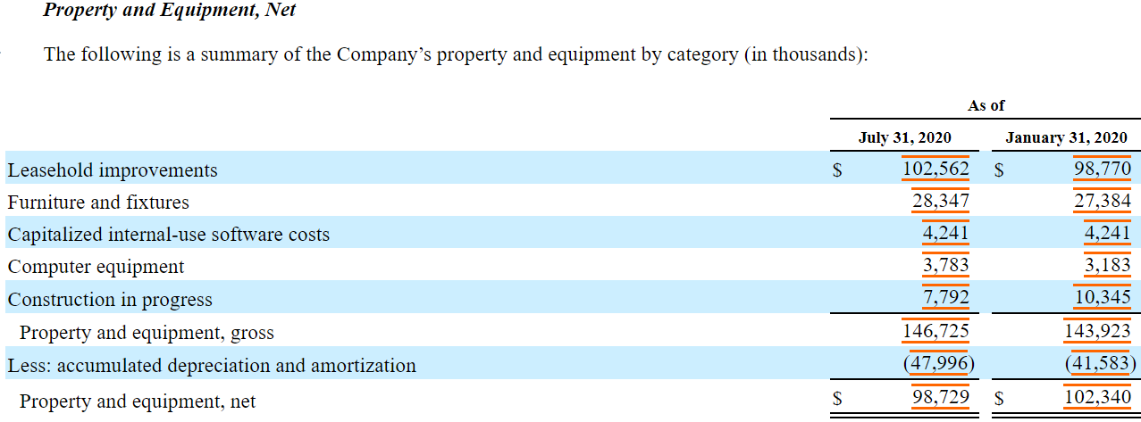
And here’s our transcribed data in Excel:
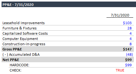
Intangibles

Here’s the relevant section in the 10-Q:

And here’s our transcribed data in Excel:

6) Hosting Commitments

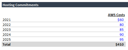
Similarly, we can find hosting commitments in the latest 10-Q. Here’s the relevant section:

From this blurb, we learn the following:

  • Slack has already spent $15 million on hosting this year ($425 - $410).
  • Slack must spend at least $60 million on hosting during Q3 and Q4 this year ($75 - $15).
  • Next year (FY 2022), Slack has a minimum AWS hosting commitment of $80 million. In FY 2023, Slack must spend $85 million on hosting, etc.
  • The minimum increases by $5 million each year.

We’re going to use these commitments as our projected hosting costs. Here’s the data in Excel:
7) Income Statement

Next, we’re going to fill in the income statement, copying Slack’s line items exactly.

Note on Process
When gathering financial data, you should always start with the most recent filings and work backwards, because the latest filings are the most up-to-date. Let’s look at an example.

You’re modeling ABC Company, which just released a 10-Q. During this past quarter, ABC Company acquired XYZ LLC, and the 10-Q financial statements include the impact of the deal. Even the financials for the prior year include XYZ LLC, since the financials are consolidated.

If you look at the prior year’s 10-Q, however, that 10-Q does not include the impact of the deal (since the deal hadn’t happened yet).

Therefore, you should pull as much data as possible from the latest filings, and you can fill in the gaps working backwards.

Let’s apply this process to the income statement:

  • We’ll start with the latest 10-Q, which includes data for Q2 2021 and Q2 2020.
  • Likewise, the prior 10-Q includes data for Q1 2021 and Q1 2020.
  • Working backwards, next we need quarterly data for Q4 2020. But – the plot thickens – there is no 10-Q for Q4. Instead we have the 10-K, which provides annual financials for FY 2020, FY 2019, and FY 2018. Save the annual data under the fiscal year columns. Here’s the annual income statement:
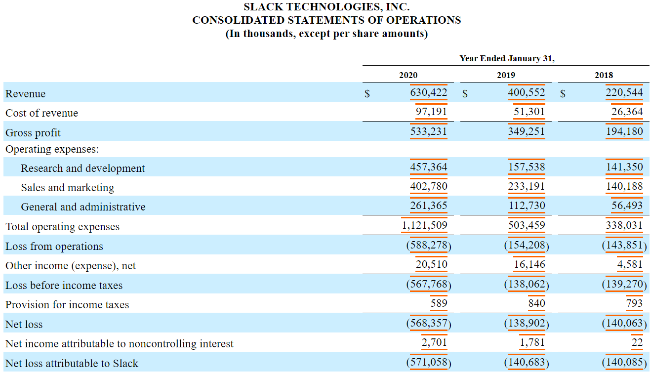
  • In addition to annual data, the 10-K also has a quarterly income statement for the preceding two years (FY 2019 and FY 2020). To find it, open the 10-K and search “quarterly results of operations.” This quarterly data extends beyond the oldest available 10-Q (Q2 2020), so we’ve captured all of the core income statement data that we have access to. Here’s the quarterly income statement from the 10-K:
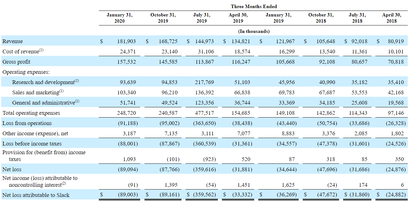
Here’s what our updated income statement section looks like in Excel:
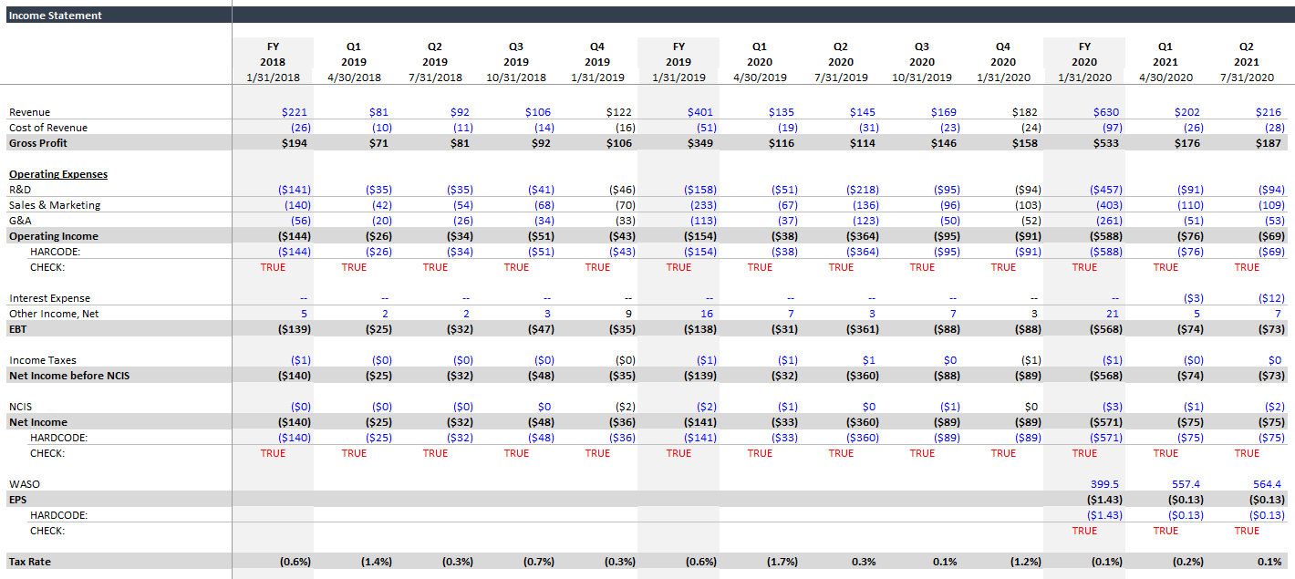
You’ll notice we included the breakdown of other income and a few extra line items. The cells shaded pink / orange are estimates.

8) Revenue Build

Now that we have historical revenue, we can turn to our revenue build. We need to pull the following data points for each time period:

  • Customer count
  • $100,000+ customer count
  • Free organizations count (they use Slack but don’t pay)
  • Percentage of revenue from customers paying $100,000+ annually

A few notes before you get started:

  • As we saw with the two most recent earnings releases (one had the free organization count, and the other did not), you won’t be able to find every data point for each period. Sometimes, the data is missing. That’s okay - we’ll work with what we have.
  • These data points, particularly the percentage of revenue, are often buried in paragraphs of text. Ctrl + F is your friend.
  • Word to the wise: Find the data points for the first couple quarters manually. Learn the words that Slack uses to describe / surround these metrics, and then search through the older filings using these keywords.

After lots of searching, you should have the following data:

We couldn’t find data for the cells shaded pink / orange, but we added estimates to some of them.

Deriving Unit Pricing & Volumes

Between the metrics above and historical revenue (from the income statement), we should be able to derive the following:

  • Revenue per big customer ($100,000+)
  • Revenue per small customer (< $100,000)

Take a minute, and try to figure out how you would calculate these values using the information available.


Okay, need a hint? Here are the rows from our revenue build:

Try to fill in those rows with the correct formulas. If you’re stuck, check out the completed Excel file.

Ultimately, this is what your revenue build section should look like:
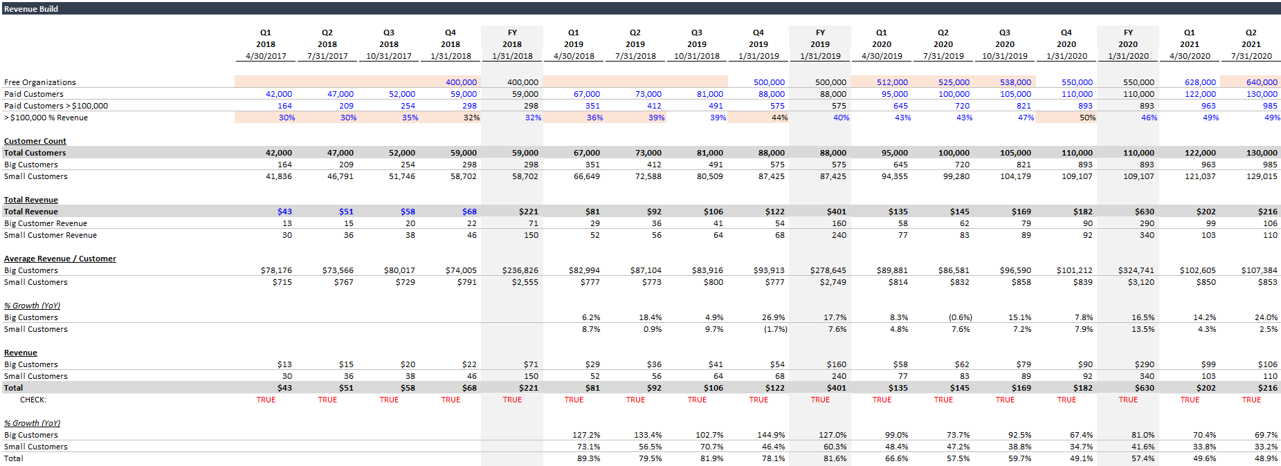
At first glance, the numbers look good. Slack’s revenue per customer increased (YoY) almost every quarter. The revenue per customer for big customers looks particularly juicy. You could interpret this in several ways:

  1. Slack grows within its largest accounts like a virus.
  2. Slack’s larger, but-still-small customers are growing rapidly, and Slack grows with them. They eventually convert from small to big.
  3. Slack is landing bigger and bigger fish.

    The truth is probably a mix of all three (and some other options we’re not thinking of).

9) Balance Sheet

The balance sheet is straightforward, but extra tedious. It’s extra tedious, because each 10-Q contains balance sheet data for the current quarter and the prior fiscal year end. This means that the Q1 and Q2 10-Qs only contain balance sheet data for three quarters combined (since both reference the same prior fiscal year end).

Alas, let’s throw on some tunes and grind it out.

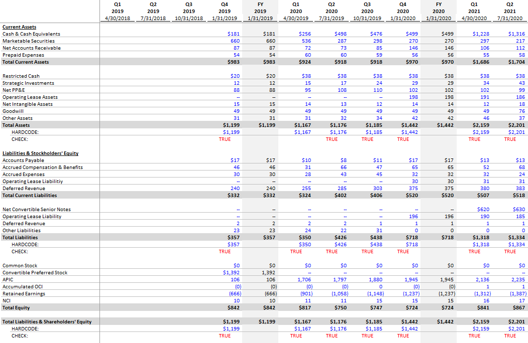
At a certain point we ran out of historical data, so our balance sheet looks a bit abbreviated compared to the income statement. Here it is:
Pro Tip: Use Footnotes
We were lazy and didn’t add footnotes to our historical data. Don’t do that. At the very least, each hard-coded number should include the URL for the relevant filing. That way, if you need to find the source, you can pop open the relevant filing and Ctrl + F for the number.

Aside: On Balance Sheets
When building standalone models, a lot of people skip the balance sheet or simplify it. If you’re working on high-level banker outputs, sure, I get it. But if you’re an investor, use the real thing. Learn what each line item represents. As an investor, it’s important to monitor the balance sheet and think critically about what’s being capitalized and whether it’s appropriate.

10) Statement of Cash Flows

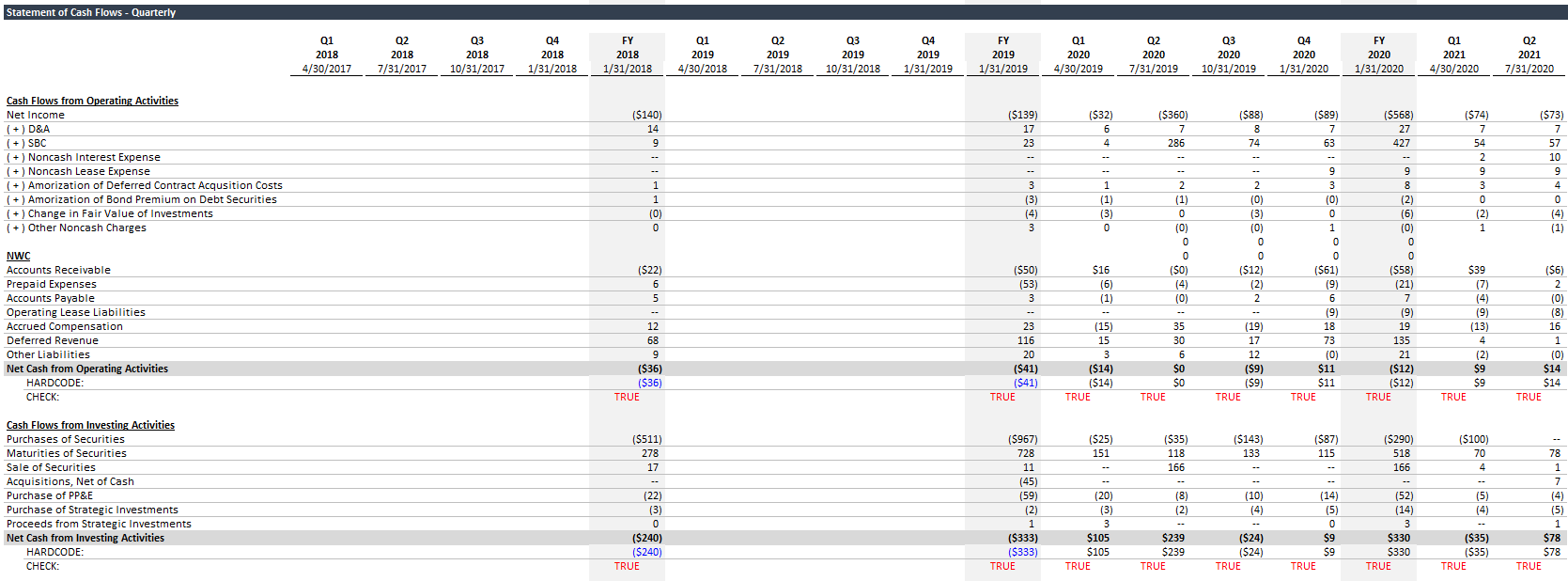
Last but not least, we need the statement of cash flows. We’re actually going to split this into two sections due to a reporting complication: 10-Qs show cash flow data on a cumulative basis. This means Q1 contains the cash flows for the three months of Q1. But Q2 contains combined cash flows for Q1 + Q2, and Q3 contains cash flows for Q1 + Q2 + Q3.

To remedy this, and calculate a quarterly statement of cash flows, we need two copies of the statement of cash flows. The first copy will consist of the data as reported. The next copy will be our quarterly output. Once we have the raw data, calculating the quarterly figures is straightforward:

  • Q1 calculated = Q1 as reported.
  • Q2 calculated = Q2 as reported - Q1 as reported.
  • Q3 calculated = Q3 as reported - Q2 as reported.
  • Q4 calculated = Annual as reported - Q3 as reported.

Now that you know the workflow, let’s throw on some tunes and get going.


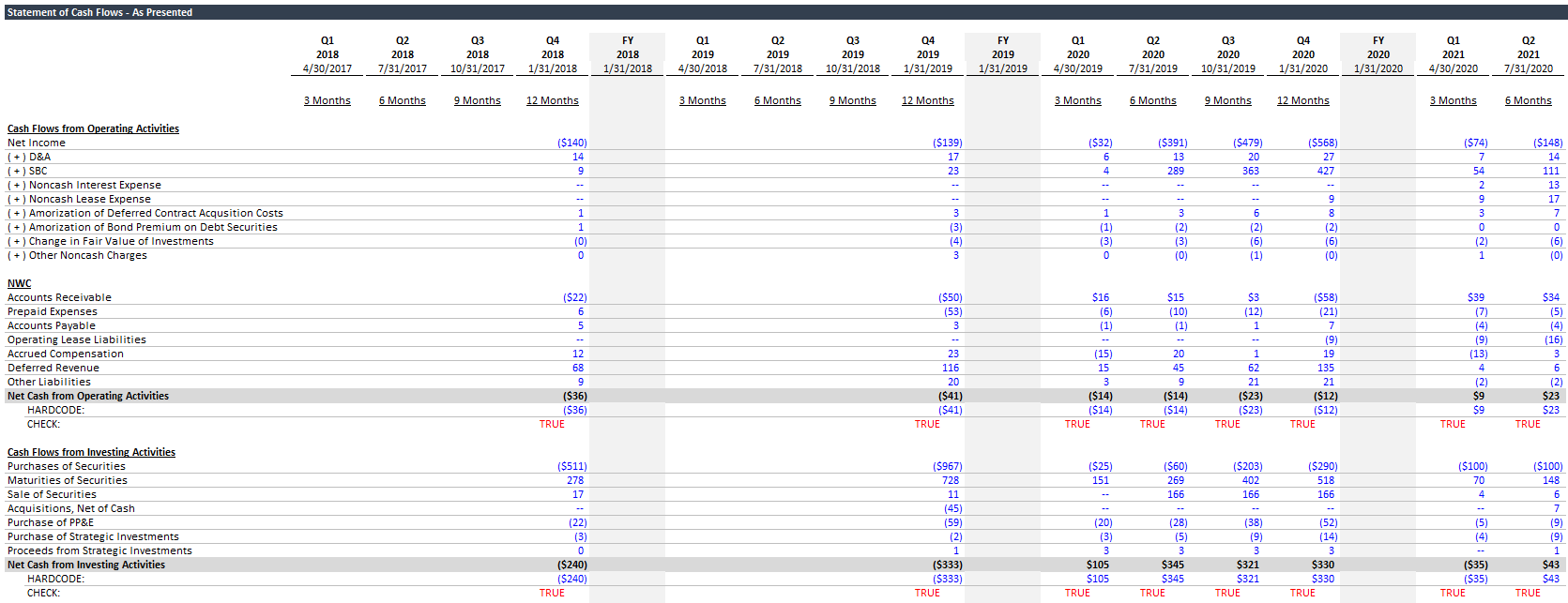
Here’s the statement of cash flows as reported:
And here’s the quarterly statement of cash flows:
Pro Tip: Working Capital Comparison
In our standalone model, we’ll be projecting working capital using balance sheet / income statement ratios (e.g., Days Sales Outstanding). We’ll derive these ratios by comparing historical income statement and balance sheet data.

You should always compare balance sheet working capital changes to values reported in the statement of cash flows. Why? Because if the numbers aren’t close, that means the company is stuffing other items into the working capital lines in the statement of cash flows. Therefore, your projections won’t capture the stuffed items (because you’re using balance sheet and income statement data for the projections), and your projected line items won’t really be comparable to the historical values. This is nightmare fuel for a financial analyst, and there’s not an easy remedy.

Fortunately, we checked, and Slack’s balance sheet changes at least approximate the values reported in the statement of cash flows. Nice job, Slack! Feel free to compare the two and check for yourself:

  1. Beneath your quarterly statement of cash flows, add some placeholder lines for the balance sheet working capital changes.
  2. In that space, calculate the changes in balance sheet working capital lines quarter-by-quarter. For example, the change in Net Accounts Receivable = beginning period Net AR - ending period Net AR. If net accounts receivable increases, that’s cash you didn’t receive this quarter, so it’s effectively a use of cash.
  3. Compare the calculated balance sheet changes to the values in your quarterly statement of cash flows. As long as they’re close, that means we’re on the right track.
  4. You should also be careful to add any related items when comparing the two. For example, if the statement of cash flows separately reports bad debt expense, that line should be added to the accounts receivable line for the comparison, since the balance sheet reports accounts receivable net of the allowance for doubtful accounts.
  5. Once you’ve checked that the working capital values roughly match, go ahead and delete the comparison calculations. They won’t be need anymore.

Conclusion

Congrats! It was a slog, but we’ve pulled Slack’s historical data, and we’re ready for the next step: building operating cases. Soon, we’ll have our standalone model.

In this tutorial, you:

  • Continued exploring the SEC EDGAR website
  • Learned how to pull historical financial data
  • Became more familiar with financial footnotes
  • Learned the framework for targeting your data search – what’s the company’s business model, and what key metrics do I need?

Reach out with any questions.

Standalone Model (Part 1) - Public Market Overview

Introduction

This will be the first in a series of articles showing you how to model a public company.

We’re going to build a standalone model for Slack Technologies, Inc. (NYSE: WORK). A standalone model is exactly what it sounds like: a financial model for a given company without any assumed transactions (e.g., acquisition, dividend recap, etc.). Oftentimes, a standalone model is the first building block in a larger financial analysis exercise. For example, if a bank is hired to help a company review its strategic alternatives, one of the first steps is working with management to build a standalone model. The standalone model serves as the company’s base case, which all strategic alternatives are then compared to.

Likewise, public markets investors model public companies in order to project financial results and evaluate investment opportunities. For private equity investors, building a rigorously tested operating model is one of the key workstreams in any deal. Knowing how to build rock-solid standalone models is a foundational skill for investment banking, private equity, and hedge fund professionals.

This article will walk you through building a public market overview (PMO), which is the first step in any standalone model for a public company. A public market overview calculates a company’s equity value and enterprise value, along with basic trading multiples.

Future articles in this series will walk you through building the full standalone model and accompanying operating cases. This is step one.

Getting Started

We recommend you start from a blank Excel workbook and try to follow the steps below. But if you prefer, here’s the completed Excel file.

1) Create Cover Tab

First, we’re going to create a cover tab. Our cover tab looks like this:

A few things to point out:

  • Below the cover area, we wrote our project code name (“WORK”) in cell F47. We’re naming this cell PROJECT.

    To name a cell, you press Ctrl + F3. When you name a cell, you can then refer to it anywhere in the workbook using its new name (in this case, PROJECT).

    Word to the wise: don’t overuse this functionality. If you have more than 10 named cells in your model, you’re doing too much.

  • The title in the cover area is actually a formula using our project code name. The formula is:

    =”Project “&PROJECT

  • Similarly, the date / timestamp below the title is created using the formula:

    =now()

2) Create PMO Tab

Next, we’re going to create a new tab for our public market overview (PMO). Again, a public market overview calculates a company’s equity value, enterprise value, and implied trading multiples. This might sound simple, but calculating equity and enterprise values can involve a surprising degree of nuance.

  • Okay, let’s create a new tab. The shortcut to create a new Excel tab is SHIFT + F11.
  • Now, let’s rename the new tab PMO. The shortcut to rename an Excel tab is: ALT > H > O > R.
  • Let’s apply some basic formatting to our new tab. In the upper leftmost cell, we’ll reference the project name again.

    = “Project “&PROJECT

  • Below the project name, let’s put a page header - in this case, “Public Market Overview (PMO)”

Your new PMO tab should look like this:

3) Add PMO Layout

Let’s add the basic structure of our PMO. Remember - we’ll be calculating equity value, enterprise value, and trading multiples for Slack.

How do we calculate equity value for a public company? Pretty simple, we multiply the number of shares by the stock price. We’ll need (i) the stock price and (ii) the fully diluted share count.

How do we calculate enterprise value for a public company? We take the equity value, and we add net debt. We’re already calculating the equity value (above), but we’ll need to look at Slack’s latest filings in order to determine the net debt.

How do we calculate trading multiples? (If you really have no idea, this is not the right tutorial series for you.) We’re going to divide equity value and enterprise value, respectively, by various financial metrics for Slack, such as revenue, EBITDA, and net income. The exact metrics and multiples we use will depend on the company’s financials.

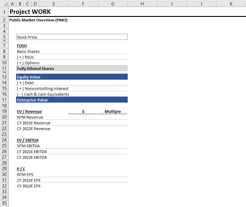
Here’s what the outline of your PMO should look like:

Stock-Based Compensation

You’ll notice that we’re adding options & RSUs to basic shares in order to calculate the fully diluted shares outstanding (FDSO). Most public companies offer some form of stock-based compensation to employees, and options and RSUs are two common varieties. When we go through Slack’s financial statements, we may discover additional share awards, or we may find out that Slack doesn’t have options or RSUs. Ultimately, we need the fully diluted share count, so that we can calculate accurate equity and enterprise values.

Some theory - why we’re focused on counting every last share…
A company’s stock price gives us the implied equity value per share. We must assume that the market is relatively efficient. Therefore, the market is doing the same basic math as us, and knows exactly how many outstanding shares there are, including from stock-based compensation. Armed with this knowledge, the market is then giving us a price, which implicitly is the most diluted (lowest) value. If we don’t include all shares in our equity value calculation, we’re undervaluing the given company, because we’re multiplying the market price (reduced by share awards) by a half-baked share count.

Noncontrolling Interest

Noncontrolling interest represents the portion of any subsidiaries not owned by Slack. For example, if Slack bought 80% of XYZ Co three years ago, all of XYZ Co’s assets, liabilities, revenues, expenses, and cash flows would be included in Slack’s consolidated financials. The outstanding 20% of XYZ Co - not owned by Slack - would be included in Slack’s balance sheet as noncontrolling interest.

Noncontrolling interest is included as a debt-like item in the build from equity to enterprise value. It’s treated like debt, because it represents a claim on Slack’s consolidated net operating assets that is not included in Slack’s equity value. Remember, the noncontrolling interest is the portion NOT owned by Slack and, therefore, not indirectly owned by Slack’s shareholders.

More theory - what does enterprise value represent?
This concept is often poorly explained. I’ll try to do a better job here. Enterprise value represents the aggregate value of a business, or collection of assets, irrespective of capital structure.

For example, when you buy a house, you fund the purchase using some combination of debt and down payment. The enterprise value for the house is the total amount of money transferred to the seller. Enterprise value ignores capital structure - it is purely a measure of aggregate value.

4) Searching the Financials

Now the fun begins. Reading and searching a company’s financials deserves its own (lengthy) article series. We’ll do our best to cover the essentials below.

SEC Filings

Since we’re evaluating a US-listed company (Slack), we’ll go to the SEC’s website to pull the filings. A lot of people are intimidated by the SEC website, due to its slightly clunky interface, but once you get the hang of it, it’s fast and easy. Personally, I feel more comfortable pulling filings directly from the source - and in the US, that’s EDGAR, the SEC’s filings website.

I never remember the website URL, so I always just google “SEC EDGAR.” The first result is the correct link. On the left side of the EDGAR webpage, you should see a search box labeled Company and Person Lookup. That’s where you enter the ticker. So let’s type in Slack’s ticker, WORK, and we’ll get going.

You should now be on Slack’s EDGAR page, and you should see “Slack Technologies, Inc.” at the top (here’s the link in case you want to double-check).

Filings are listed in reverse chronological order (most recent filings at the top), and the number-and-letter symbols in the leftmost column represent filing types. You’ll mainly be interested in 10-Ks (annual financials), 10-Qs (quarterly financials), and 8-Ks (periodic investor updates), but here’s a complete list of filing types. I wouldn’t recommend reading this list, unless you have an unanswered question. For example, if you see an unusual form code and want to know what it is, try google first. If you can’t find a succinct answer quickly, then pop open this list and Ctrl + F.

As I mentioned, 10-Ks, 10-Qs, and 8-Ks are where you’ll spend most of your time. 10-Ks provide the most comprehensive information, and they’re filed annually. You can think of 10-Qs as leaner, less filling versions of the 10-K. 10-Qs are filed quarterly. This guide on how to read a 10-K, provided by the SEC, is pretty thorough without making your eyes bleed (at least mine didn’t). If you’re new to filings research, it’s a good place to start.

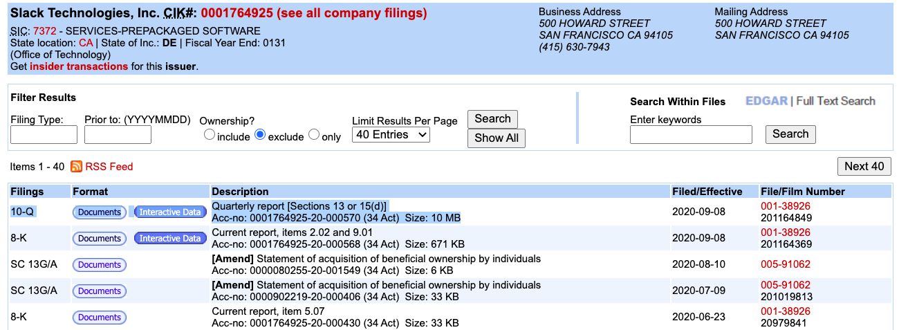
When building a PMO, you want to locate the latest 10-Q or 10-K, which should have all of the information you need. Ideally, the latest 10-Q or 10-K will be one of the first filings listed, as is the case here (as of November 25, 2020). See below:

It’s better (for you) if the latest 10-Q / 10-K is near the top of the list, because then you have to check fewer filings to ensure nothing material has changed. Remember - 8-Ks contain investor updates, so sometimes you can run into situations, in which an important 8-K is released after the latest 10-Q / 10-K. By default, you should check every filing above the latest 10-Q / 10-K, and it’s also a good idea to check any 8-Ks directly below the latest 10-Q / 10-K. You don’t want to miss something important. Anyways, we’re in luck. No subsequent 8-Ks, and the latest 10-Q should have everything we need.

10-Q and Exhibits

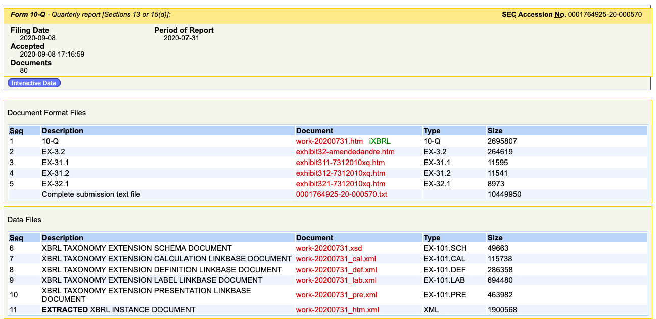
Let’s click on that top 10-Q. You should see this menu:

The first link in the table (here, it says “10-Q”) is the main filing. We’ll go to that in a second.

The exhibits listed below the filing contain various legal documents. You can ignore these unless you’re hunting for something specific. For example, the first exhibit (“EX-3.2”) contains Slack’s latest bylaws. These are the legal rules that govern the election of company directors, stockholders’ meetings, etc. If you work at an activist hedge fund, you might find these interesting. If you work at a bank, you’ll probably never read these.

Anyways, moving on. Let’s click the first link, which will give us the latest 10-Q.

Finding the Data We Need

Now, I’m going to go through and show you where to find each piece of information we need for the PMO. As we find specific pieces of information, you can add this data to your Excel file.

As a reminder, we’re looking for:

  • Basic share count
  • Dilutive equity awards
  • Total cash and cash-like items
  • Total debt and debt-like items

Basic Shares

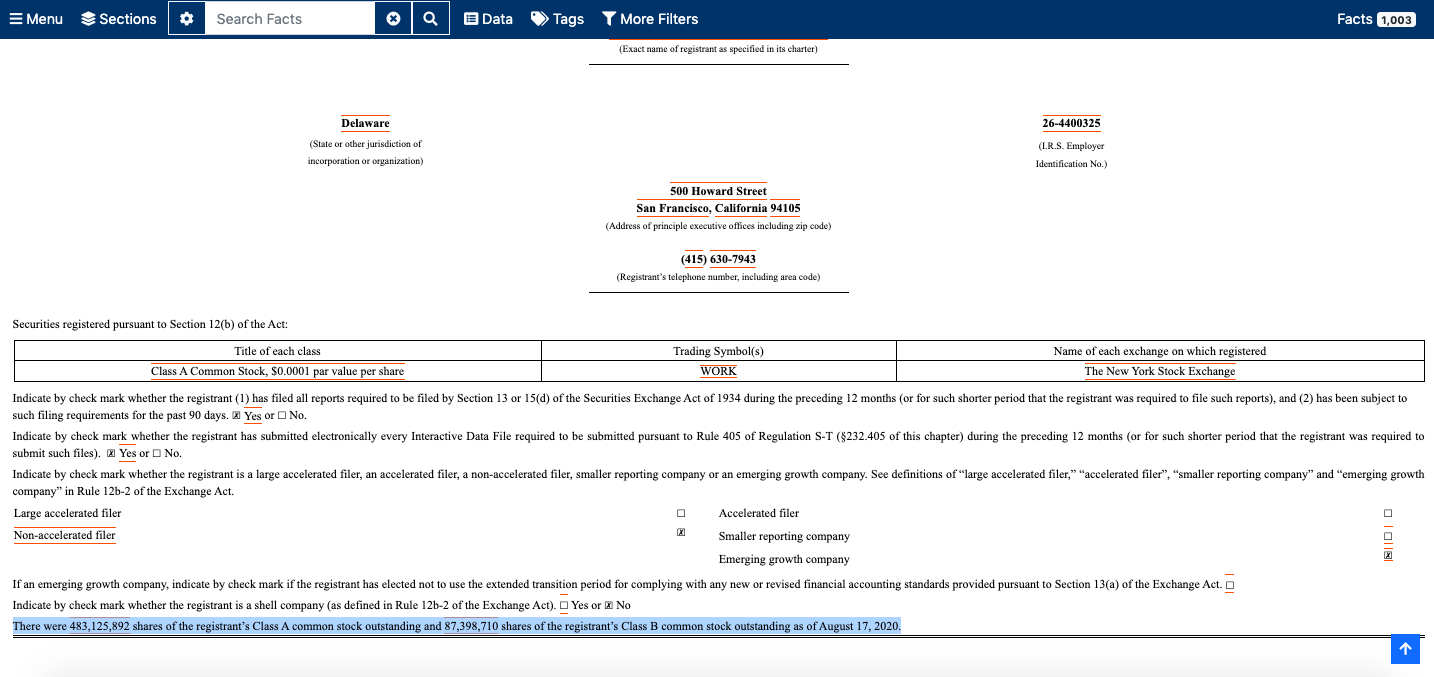
You can find the basic share count on the cover of any 10-Q / 10-K. This is not the fully diluted number and doesn’t include stock-based compensation. See below:

It looks like Slack has two classes of common stock: Class A common stock and Class B common stock. We’ll need to confirm, but my guess is that the only difference between the two classes is voting rights. The class B shares likely command more votes per share.

Let’s record both values below our PMO for the time being.

Balance Sheet

Cash

If we continue scrolling through the 10-Q, soon we’ll come to the balance sheet. Note: 10-Qs don’t have as much fluff as 10-Ks. If you’re scrolling through a 10-K, it might take you a little while to get to the balance sheet. The page down key is your friend.

Every balance sheet should include a cash and cash-equivalents line item under current assets. But we still need to read the rest of the balance sheet to ensure we’re not missing anything.

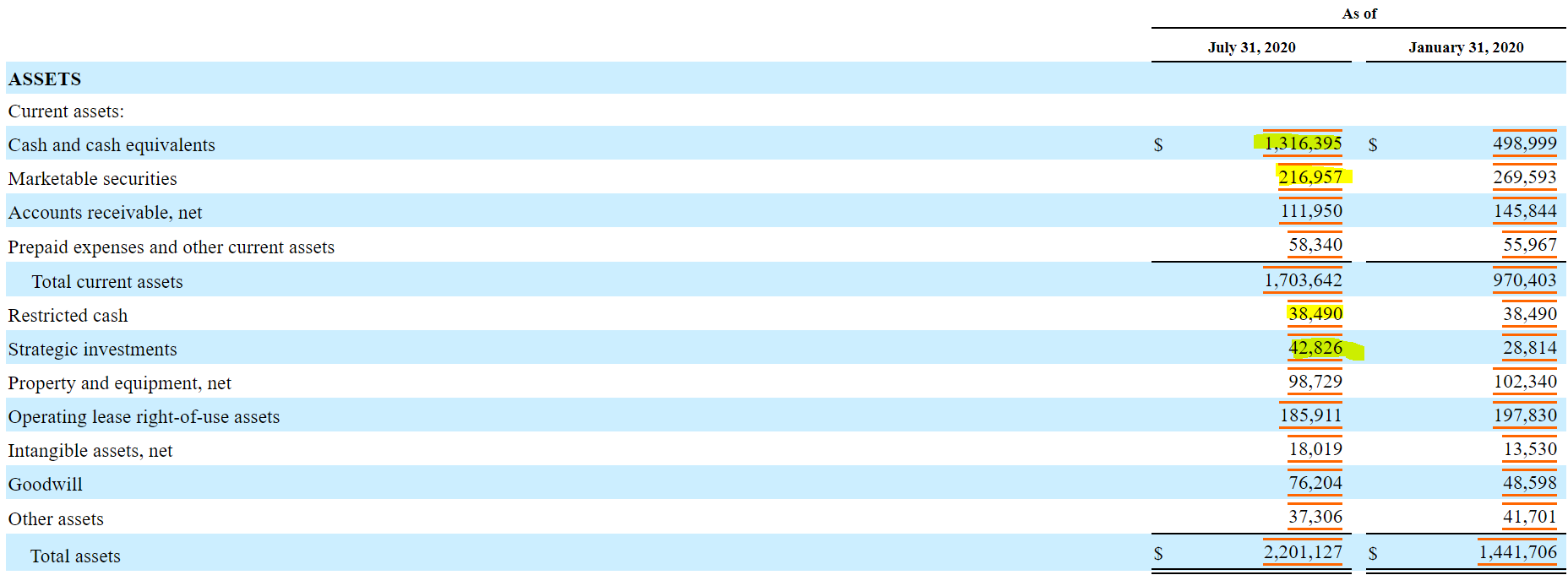
I see four line items we might want to treat as cash ($ in millions):

  • Cash and cash-equivalents ($1,316.395)
  • Marketable securities ($216.957)
  • Restricted cash ($38.49)
  • Strategic investments ($42.826)

Cash and cash-equivalents is obviously cash, and marketable securities should likely be included as well. For restricted cash and strategic investments, we’ll need to read the footnotes to confirm.

Debt

Before we move on from the balance sheet, let’s identify any debt and debt-like items.

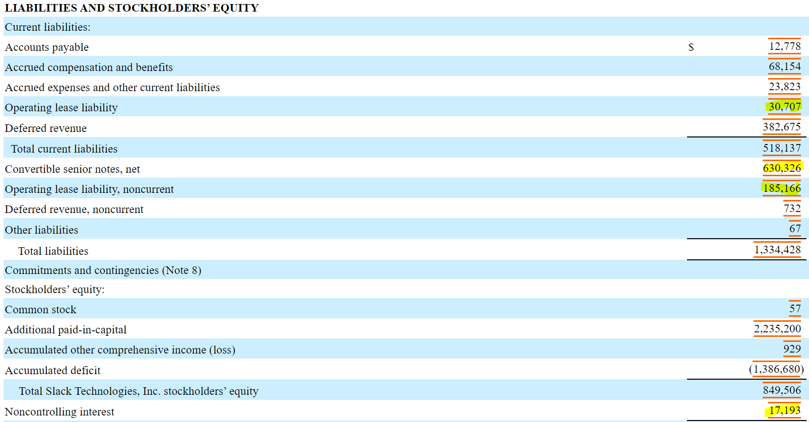
I see several line items we want to include ($ in millions):

  • Operating lease liability, current & noncurrent ($215.873)
  • Convertible senior notes ($630.326)
  • Noncontrolling interest ($17.193)

We’ll need to read more about the operating lease liability and the senior notes. We already discussed why we’re including noncontrolling interest (above).

Income Statement

Now, we can continue scrolling through the document. Glancing at the income statement, we see that Slack has negative operating income, net income, and earnings per share. Therefore, we can delete the EV / EBITDA and P / E multiples from our PMO. Slack’s stock obviously doesn’t trade based on negative multiples. Some industry knowledge confirms this - growth SaaS businesses trade on forward revenue multiples.

SaaS stands for Software as a Service. Here’s a good primer from Salesforce on the SaaS business model.

Into the Footnotes

After adjusting our PMO template, let’s keep scrolling down. Once you get past the financial statements, you’re into the footnotes. In books or the academic setting, footnotes usually contain references or extraneous information. But for financial analysis, footnotes are the most valuable source of information.

Accounting Policies

Usually, one of the first notes is a description of important accounting policies. For public markets investors, this is a must-read section. Accounting gives you a lot of leeway to smooth earnings and game the system. You should read the accounting policies with a skeptical eye to understand what accounting decisions management is making and where they’re applying judgement.

I usually skim this section, but right away I see something useful for our PMO:

The face value of the senior notes is 862.5 million, versus the lower amount on the balance sheet. The balance sheet figure must contain a substantial discount. The blurb in the accounting policies also tells us which footnote has more info (note 7).

Fair Value Measurements

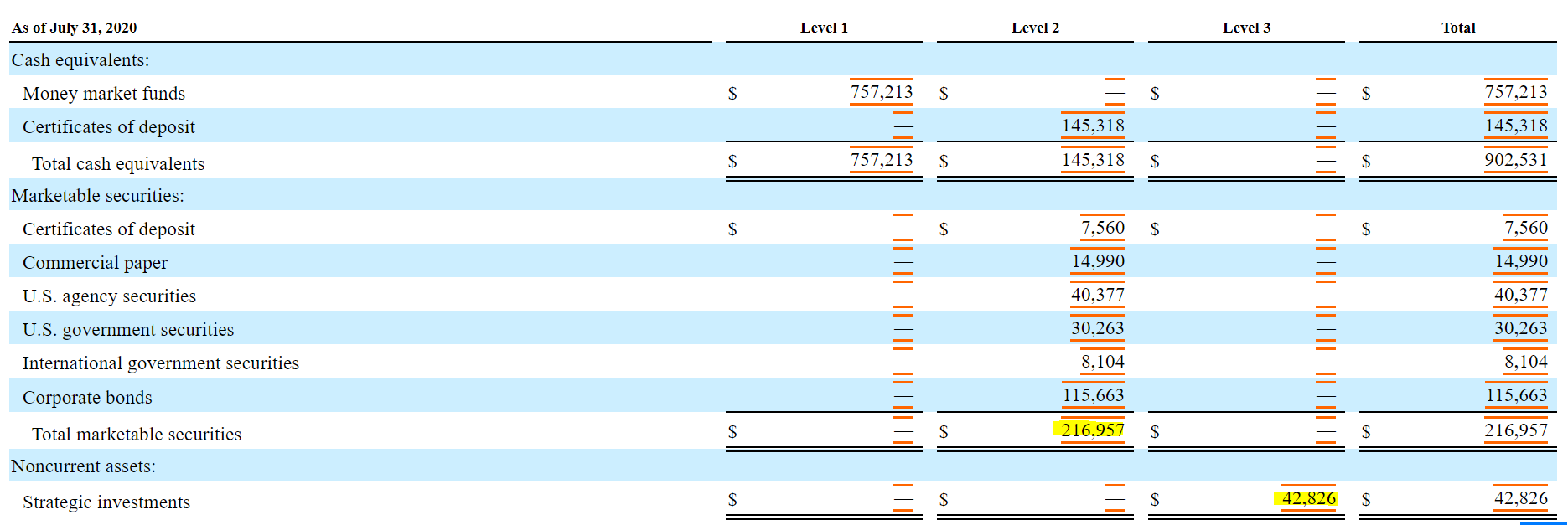
Continuing to scroll through the footnotes, we come to the Fair Value Measurements section, which details assets recorded at fair value instead of cost. This includes the extra line items we’re considering including as cash-equivalents.

You can see that the marketable securities line item consists of fairly liquid assets: corporate bonds, US government securities, etc. We can treat marketable securities as cash.

Strategic investments, on the other hand, are highly illiquid. Therefore, we will NOT include that line item as cash.

Business Combination

Next, we see a note about Slack’s recent acquisition of Rimeto Inc. It is worth reading any Business Combination notes, because sometimes 10-Qs and 10-Ks include basic financial information for acquisitions that occurred after the balance sheet date. In those cases, the acquired company is not included in the consolidated balance sheet, and we would need to add any acquired cash to the previously noted amounts, etc. Fortunately, the acquisition of Rimeto was completed on June 29 - well before the balance sheet date (July 31).

Operating Leases

Eventually we’ll come to the Operating Leases section. As you’ll recall, we noted an operating lease liability on the balance sheet as one of the potential debt-like items, so let’s read this section.

In this case, it looks like the operating lease liability is debt-like, and we should include it in our enterprise value calculation. It is the implied debt financing required to own the leased assets. Historically, leases have been an accounting subject prone to trickery. Some companies use capital leases (effectively, debt + leased assets on the balance sheet); other companies use operating leases to appear asset-light. Capitalizing the operating leases levels the playing field and makes comparison between companies somewhat easier. FASB’s new lease accounting standard (ASC 842) reduces some of the mischief in lease accounting.

Debt

The next section covers Debt and Financing Arrangements. We definitely want to read this.

Right away, we receive confirmation that the face value of notes is 862.5 million.

We also learn that the notes are convertible to common stock. That means, layered within the debt instrument, is an option for the debtholders to exchange their notes for stock. This requires further inspection, because this debt could increase our diluted share count.

We learn more about the conversion option below:

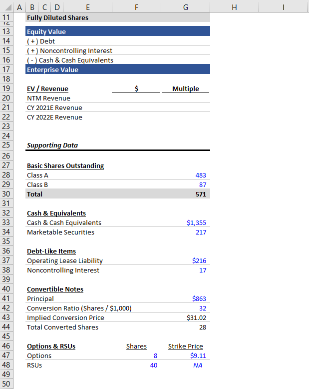
This means that every $1,000 of debt can be exchanged for 32.2630 shares. If the stock price is greater than $31, we should assume the debt converts to shares, and if the stock price is less than $31, we can treat the notes as normal debt. We’ll need to add a row to the diluted shares section of our PMO to account for the conversion option. We can label this new row: “ITM Convertible Notes” (ITM stands for in the money).

We also learn that Slack has a revolving credit facility.

But it’s completely undrawn:

Commitments and Contingencies

The next section is Commitments and Contingencies. The first blurb tells us that restricted cash ($38.5 million) consists of standby letters of credit for operating leases. Standby letters of credit are essentially cash set aside and guaranteed, by a bank, for payment to a third party. It sounds like these letters of credit are essentially prepaid deposits for lessors. Since we’re counting operating lease liabilities as debt (in our enterprise value calculation), we should also include the corresponding restricted cash. It doesn’t make sense to include one and not the other. By the same logic, if you choose not to include operating lease liabilities as debt, you should not include restricted cash, since it is tied to the leases.

Note on Restricted Cash: As an astute reader pointed out, restricted cash is presented separately on the balance sheet for good reason. Usually, you would not include it in net debt. We had to read the footnotes to discover that it is tied to operating lease liabilities, and therefore, it should be included in our enterprise value calculation. Lenders, however, would not give the company credit for restricted cash, because it’s not generally available to the company - it’s subject to a prior legal claim (operating leases).

Pro Tip: In this tutorial, we’re reading the notes sequentially. But your process doesn’t need to be linear. For example, if you see an odd line item on the balance sheet, you can CTNL + F for more detail.

Checking In

Before continuing to read the notes, let’s assess what we still need to find.

  • We have cash and cash-like items.
  • We have debt and debt-like items.
  • We have basic shares.
  • We still need to find any dilutive securities, such as stock options.

Stockholders’ Equity

We eventually come to note 9 - Stockholders’ Equity. This section details outstanding options, RSUs, etc.

You’ll notice that there are multiple option counts we could potentially include. I’ll make it simple for you. Always use the total number of outstanding options. You can ignore the vested counts.

In our PMO tab, we’ll record 8.092 million options with a weighted-average strike price of $9.11.

Below the options table, we see a section on Restricted Stock Units and Restricted Stock Awards. These two types of compensation sound similar, but are quite different. Here’s a good overview on the difference between RSUs and RSAs. Essentially, RSUs are not actual shares. They represent a promise to receive shares in the future. But RSAs are full shares, subject to vesting and certain restrictions. Whereas RSUs are not included in the basic share count, since they’re not real shares, RSAs are already part of the basic share count. Therefore, we will add RSUs to the basic share count in order to calculate fully diluted shares outstanding, but we can ignore RSAs since they are already included.

After recording the options and RSUs, we have all the historical information we need for our PMO. At this point, your updated PMO tab should have the following data:

5) Calculate Equity Value

Now we’ll calculate Slack’s equity value.

First, we need a stock price. On November 25, Slack’s stock price rocketed due to acquisition rumors. Therefore, we’ll use the closing stock price on November 24 ($29.58) as our unaffected price.

Next, we need to calculate the diluted shares outstanding.

We can link to the basic share count and RSU count from our supporting data. But we’re going to calculate the net shares from options using the Treasury Stock Method, which relies on the stock price.

Treasury Stock Method

The Treasury Stock Method sounds fancy, but it’s pretty simple. In plain English, the Treasury Stock Method calculates how many options would be exercised at the given stock price. Then, it takes the proceeds from exercised options (the cash paid to convert options to shares) and assumes those proceeds are used to repurchase shares, in order to minimize dilution. The Treasury Stock Method provides the net shares (the number of options exercised, less the number of shares repurchased using option proceeds).

How ‘bout a formula?

= number of options - (option strike price x number of options) / stock price

Remember, we’re taking the number of options exercised. Then, we’re calculating the proceeds from exercising those options (option strike price x number of options). We divide the proceeds by the stock price in order to calculate how many shares can be repurchased.

So the number of net shares equals (i) the number of options exercised, less (ii) the option proceeds divided by the stock price.

Simplified further:

= number of options x (1 - (strike price / stock price))

Try to calculate the net new shares from Slack’s options using this formula. You should be getting 5.59 million new shares.

Convertible Debt

As we discovered in our filings research, Slack has convertible notes. These can be counted as either debt (included in net debt) or additional shares (assuming the debt converted to equity). Therefore, we’ll need to account for the convertible debt in both the diluted shares and net debt.

Here’s what we came up for the diluted shares portion:

= if (stock price > implied conversion price, total converted shares, 0)

Since the unaffected stock price is less than the implied conversion price, the debt should not be converted to equity (it’s worth more as debt).

In summary, the diluted share count consists of basic shares, plus RSUs, plus options (calculated using the Treasury Stock Method), plus any converted shares.

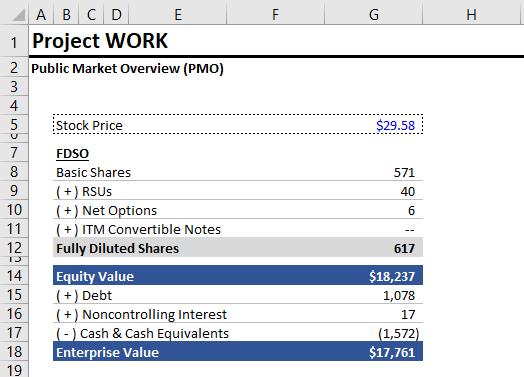
Our equity value is simply the diluted share count multiplied by the stock price ($18,237 million).

6) Calculate Enterprise Value

Now that we have the equity value, the hard part is over. The enterprise value is the sum of (i) the equity value, (ii) total debt, and (iii) noncontrolling interest, less cash and cash equivalents.

We can link the noncontrolling interest value from our supporting data below. Likewise, the cash and cash equivalents value is the sum of cash and marketable securities ($1,572 million).

The debt balance contains the only wrinkle. Again, we need to account for the conversion feature of the debt. If the debt is converted, then the notes will cease to exist. Therefore, our debt balance formula is:

= operating lease liabilities + if (stock price > implied conversion price, 0, debt principal amount)

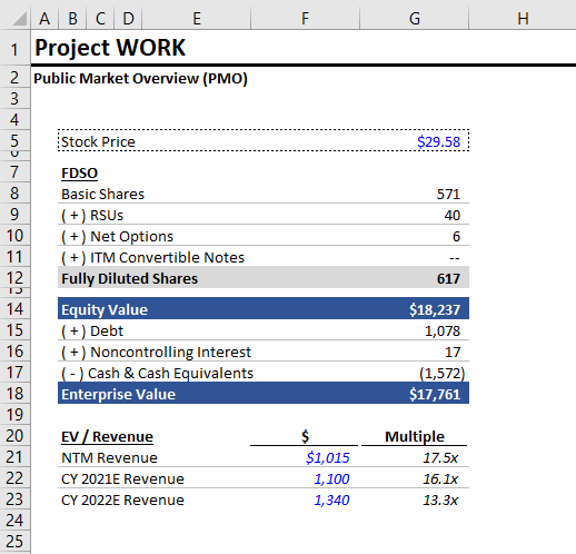
You should have a debt balance of $1,078 million and an enterprise value of $17,761 million. The enterprise value is less than the equity value, which may seem strange, but just means that the company has more cash than debt.

Here’s what the completed equity value and enterprise value calculations should look like:

7) Calculate Trading Multiples

Last, we need to calculate the implied trading multiples. We removed the EBITDA and EPS sections, so we’ll only be calculating the enterprise value / revenue multiples.

Here, you could pull consensus estimates for revenue from a data service, like Bloomberg, CapIQ, or FactSet. In future articles, we’ll pull the forward revenue numbers from our operating model. In the meantime, we’re going to use placeholder numbers:

  • For NTM revenue, use $1,015 million.
  • For CY 2021E revenue, use $1,100 million.
  • For CY 2022E revenue, use $1,340 million.

At this point, calculating the revenue multiples should be easy. Divide the enterprise value by each revenue figure. This is what your completed PMO should look like:

Here is the completed PMO Excel file.

Conclusion

Congrats! You successfully built a public market overview (PMO) for Slack. You have:

  • Explored the SEC EDGAR website
  • Learned the basics of filings research
  • Learned about different types of equity compensation
  • Learned the Treasury Stock Method
  • Reinforced your understanding of enterprise value and calculating enterprise values for public companies

We’re going to continue this series by building a full standalone model for Slack, complete with flexible operating cases. The next step is pulling Slack’s historical financial and operating data.

Reach out with any questions.

Payment-In-Kind (PIK) Interest

Introduction

This will be a quick post covering Payment-In-Kind (PIK) interest. PIK interest is a feature of some debt instruments that allows the interest expense to be accrued, rather than paid in cash, for a certain number of years. This is where the name payment-in-kind comes from - the interest expense on the debt is paid in kind, i.e., with more debt.

Historical Context

While rare today, PIK interest was relatively common during the run-up to the 2008 financial crisis, and therefore, it is often seen as a symptom of loose credit markets and boom times. Many prominent 2006 and 2007 private equity deals had debt instruments with PIK interest. Some of these deals did not go well.

Why Do We Care?

  • PIK interest is uncommon today, but it still pops up occasionally.
  • PIK interest is often associated with private equity, since it allows companies to support a bigger debt burden upfront and then gradually delever.
  • Even if most private equity professionals never issue debt with PIK interest, it’s almost mandatory to be familiar with PIK interest and understand how it works.
  • PIK interest is often included in modeling tests and private equity interviews as an extra little gotcha, which is silly, because it’s very rarely part of the job.

Why PIK Interest Is Appealing

To illustrate why PIK interest exists, let’s explore a hypothetical scenario:

  • You’re running a private equity deal, and you’re in the process of arranging financing.
  • You’re buying the target business for 1.0bn (10.0x LTM EBITDA).
  • You have bank financing lined up for 3.0x leverage.
  • The company can issue notes for an additional 3.0x leverage.
  • So together, the bank financing and the notes get you to 6.0x total leverage, and let’s assume a PF interest coverage ratio of 2.40x.
  • At this point, the private equity firm will be investing 400mm of equity (1.0bn transaction value - 600mm of debt). The projected returns are good, but not breathtaking.
  • Unfortunately, your PF interest coverage ratio is already 2.40x, so it’s infeasible to raise additional debt.
  • But the company has strong cash flows and solid growth prospects.
  • What if you could raise more debt and delay the interest payments?

PIK interest has entered the chat.

  • The private equity firm arranges an additional 100mm of junior notes, with a 3-year PIK (no cash interest expense for 3 years). These junior notes are expensive, because they’re the riskiest debt tranche in the capital structure, but they enable the private equity firm to invest less equity, which dramatically improves the projected returns.
  • Furthermore, the company has 3 years to pay down its bank debt (and reduce its interest expense burden) before the junior note’s cash interest expense kicks in.

Takeaways

  • PIK interest acts as a smoothing mechanism - moving some of the initial interest expense burden to later on. Much like a construction loan, interest expense is delayed and accrues.
  • PIK interest enables companies to support a higher initial debt burden than they otherwise could.
  • More debt, in the context of a LBO, means a lower equity investment and higher returns.

That’s why private equity professionals geek out over PIK interest - it’s quintessential 2007-era financial engineering.

How do we model PIK interest?

So now we know what PIK interest is and why it’s theoretically useful. How do we model it?

We’re going to be referring to the completed Excel template from our intermediate LBO tutorial.

This template already has PIK interest functionality built in, and we’re going to be explaining the different components in detail. We’re going to focus exclusively on the LBO_Final tab. The other tabs are intermediate steps explained in the tutorial.

1. Financing Assumptions

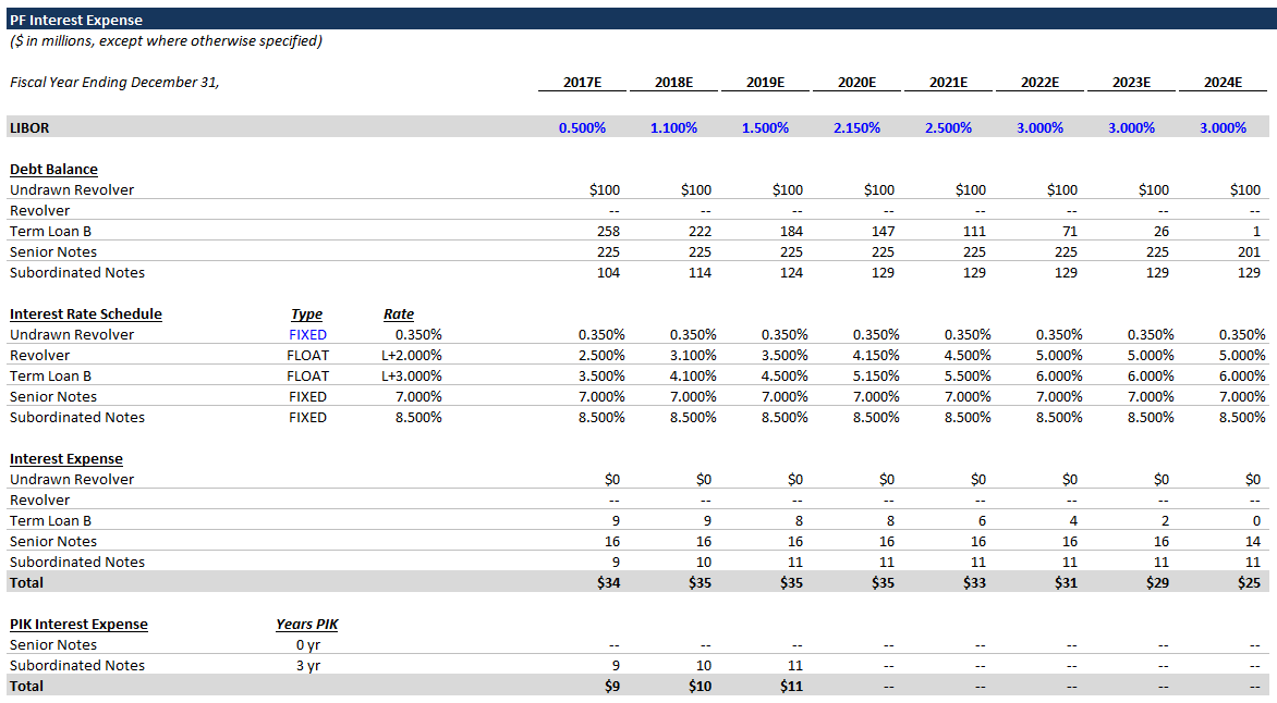
At the top of the LBO, you can see the financing assumptions, where we include a Years PIK column for each debt tranche. This column specifies the number of years of PIK interest.

We’re assuming the subordinated notes have a 3-year PIK.

2. Debt Schedule

  • When adding PIK interest to a model, build your debt schedule assuming no PIK interest at first.
  • Generally speaking, only notes have PIK interest, and since notes are not amortized each year, the ending balance for your notes should be constant. (When we add the PIK interest, the ending balance for the notes will increase, since the interest expense during the PIK period is being accrued)

3. Interest Expense Schedule

  • Likewise, build your interest expense schedule assuming no PIK interest. Although cash interest expense will change when we add the PIK functionality, total interest expense will not change. We still have to include PIK interest in the income statement, etc.
  • Below the normal interest expense schedule, add a memo section for PIK interest. The calculations for this memo section are simple:

    PIK Calculations
    PIK Interest = IF(year count <= PIK years, include interest expense, 0)

  • Remember PIK interest is a noncash expense, since it’s being paid with more debt instead of cash.

4. Add PIK Interest to Debt Balance

  • Now that we’ve calculated the PIK interest, we’re going to add it back to the debt balance.
  • We’ll revise the ending debt balance calculation for our notes to be:

    Ending Debt Balance (for notes) = Prior Period Balance - Mandatory Amortization - Optional Prepayment + PIK Interest

5. Include Noncash Interest Expense in Statement of Cashflows

We must add back noncash interest expense in the statement of cash flows, since our net income includes all interest expense (noncash + cash interest expense). In the LBO model, PIK interest is the primary component of noncash interest expense.

Conclusion

Now you should understand what PIK interest is, why private equity professionals like it, and how to model it.

Any discussion of PIK interest, however, would be remiss if it didn’t address the risks.

Risks

PIK interest is very risky. PIK interest allows a company to increase its debt burden in the near-term and pay more interest expense later on. In order for this to work, the company must be able to delever and then service the increased cash interest expense when the PIK period expires.

Furthermore, because PIK interest is riskier and is often associated with more aggressive capital structures, debt tranches with PIK interest are often expensive. Going back to our capital structure first principles, if the cost of debt is greater than the ROA, the incremental debt will actually decrease the return to shareholders. To put this in concrete terms, if we examine some of the 2007-era private equity deals that featured PIK interest, the cost of debt (with PIK interest) was sometimes greater than 12%. During the financial crisis, the ROA for many of these companies dropped well below 12%. Therefore, even when the companies managed to service their debt burden, these notes were not accretive to shareholder value.

To put it simply, PIK interest is an extremely aggressive feature, where everything has to go right for the private equity investor to win.

Next Steps

If you haven’t worked through our intermediate LBO tutorial yet, that’s a great place to start.

We also have a comprehensive (and free!) private equity modeling course.

Paper LBO Credit Terms

Introduction

This post is a continuation of our prior two articles on paper LBOs:

A couple of our readers asked how to come up with reasonable debt financing assumptions if none are provided.

In our experience, this rarely occurs. The point of a paper LBO is to assess your understanding of basic LBO mechanics, not credit markets. Furthermore, many private equity firms have dedicated capital markets professionals, who provide guidance on financing assumptions and liaise with banks. To be frank, your interviewer probably wasn’t a capital markets banker and likely has a surface-level understanding of debt financing.

That being said, the question can come up. As we started writing an addendum to our paper LBO guide, we realized this question deserves its own post. So here goes:

Understand What They’re Testing

Asking you to come up with debt financing assumptions tests the following:

  • Do you have a basic understanding of credit markets?
  • Do you have a sense for reasonable LBO financing limits? (If you’ve done a few sellside M&A pitches, you should)
  • Are you familiar with basic credit ratios?
  • Do you understand what attributes make an attractive credit?

Before composing a response, let’s review each of these topics.

Credit Markets

A market is where buyers and sellers meet to exchange goods and services.

Capital markets are a market, like any other. There are many different providers of capital, who have unique return requirements and risk thresholds. Credit markets are a subset of the broader capital markets.

Private equity firms frequently access the credit markets in order to raise debt financing for portfolio companies and new investments. Many of the larger private equity firms even have debt financing arms.

Our Intermediate LBO Guide has more detail on LBO financing and includes links to debt primers.

What makes a good credit?

Many of the attributes that make a good equity investment make a good credit investment:

  • Predictable, recurring revenues & cash flows
  • High margins
  • Performs well during recession
  • Diversified customer base / low customer concentration
  • Low - negative working capital cycle
  • Must-have product
  • Strong management team
  • Barriers to entry
  • Non-cyclical industry

Credit-Specific Factors

  • Valuable collateral or fixed assets with resale value
  • Large equity cushion (will get wiped out before debt in bankruptcy)
  • Prior credit history (how quickly has the company delevered, etc.)

To further develop your intuition around capital structure, check out our first principles guide.

Basic Credit Ratios

There are two main types of credit ratios:

  • Leverage ratios - compare the amount of debt and the company’s cash flow (EBITDA).
  • Interest coverage ratios - compare the company’s cash flow (EBITDA) and the interest expense burden.

Leverage

The two main leverage ratios are:

  • Total Debt / EBITDA
  • Net Debt / EBITDA

Interest Coverage

The main interest coverage ratios are:

  • EBITDA / Interest Expense
  • EBITDA - CapEx / Interest Expense (this is especially important for capital-intensive industries)

Why use EBITDA vs. unlevered free cash flow?
We use EBITDA for credit metrics by convention. It’s just something that the credit markets have come to accept and expect. In practice, the EBITDA used would be heavily adjusted, as defined in the credit agreements. Also, while EBITDA and unlevered operating cash flow should be relatively close, unlevered free cash flow includes the impact of CapEx, whereas EBITDA does not.

LBO Financing Limits

Rarely does an LBO exceed 6.0x leverage (total debt / EBITDA). You occasionally see deals with 7.0x leverage, but that’s aggressive.

As a rule of thumb, the interest coverage ratio should be > 2.0x. Obviously, the higher the interest coverage ratio, the better.

Finally, any private equity investment should include a minimum 20% equity. Typically, equity is 20 - 40% of total capital.

Note: The above commentary around equity percentage is a generalization. This generalization holds for generic LBO deals. More growth-oriented investments can have a much higher equity percentage, because the returns are less dependent on capital structure (the asset’s ROA is higher).


Now that we’ve reviewed the topics that this question tests, we can begin to formulate a response.

1) Ask for More Info

First, I think it’s worth asking the interviewer for more information. It shows you’re approaching the problem the right way. After all, investing and the diligence process are all about asking questions and updating your view with new information. Ask for more information about the company and the industry, as these details inform the company’s creditworthiness.

  • What industry is the company in? What does it do?

Of course, the interviewer might cut you off and say you have to work with the information already provided. If so, proceed to step 2 (below).

If the interviewer is playing along, and you’re unfamiliar with the industry, you should try to learn more:

  • Is it capital-intensive?
  • Is it a cyclical industry?
  • Etc.

If you’re already familiar with the industry, you should signal you understand some of the credit factors. For example, you might say, “Airlines are highly cyclical, so I’m going to be cautious and assume a less aggressive debt package.”

2) State Your Assumptions

Next, you should state your assumptions, so the interviewer can see how you’re thinking about the problem. This also gives the interviewer a chance to correct your assumptions and provide more information.

You can summarize what you know so far. For example:

  • Well, so far I know it’s a specialty manufacturing company based in the U.S.
  • I’m going to assume it has a diversified customer base and is relatively recession-resistant.
  • Also, I’ll assume it has ample fixed assets that will serve as collateral.
  • Based on the provided financials, it has a 25% EBITDA margin and is not too capital-intensive.

Going back to our Paper LBO Example, you were only given 2021 cash flow, not EBITDA, so you might say, “For the purposes of calculating credit ratios, I’ll assume that 2020 EBITDA = 2021 Unlevered FCF.”

3) Determine Debt Limits

Next, you need to figure out the various limits on how much debt the company can raise.

Let’s continue using our Paper LBO Example. We’re assuming 2020 EBITDA = 2021 Unlevered FCF (150).

Total Leverage

6.0x total leverage equals 900 of debt. Remember the transaction value was 1,100, so that’s too high.

Equity Percent

75% debt equals 825 of debt. That leaves 275 of equity.

Interest Coverage

In order to calculate interest coverage ratios, we need to know the interest rates of various debt tranches, so we’ll save this constraint as a confirmatory check for the end.

Combining the leverage and equity constraints, you might say: “800 total debt results in 27% equity and 5.3x total leverage, which seems reasonable.”

If there are credit concerns, you might settle on a lower total debt figure.

4) Come Up with Tranches

Contrary to our Paper LBO Example, private equity deals usually involve multiple tranches of debt. Again, for more detail on the various types of debt, you can check out the debt primers referenced in our Intermediate LBO Guide.

Here, given you don’t have much information, and this is a highly illustrative example, I think it’s best to play it safe. A classic financing scenario for LBOs is ~50% senior secured bank debt and ~50% notes (or bonds). The senior secured debt has priority and is secured against the company’s collateral, so it has a much lower interest cost. The notes have a higher interest cost, because they are junior to the bank debt.

You might say, “I’ll assume the company raises 3.0x of senior secured bank debt and finances the rest with notes. So the company raises 450 of senior secured bank debt and 350 of notes. Let’s assume the interest rate for the bank debt is Libor + 350 bps, and the interest rate for the notes is 8.000%.”

If your interviewer presses you and says that notes aren’t an option, you could finance the remainder with mezzanine debt (more expensive junior debt). An illustrative interest rate for the mezzanine debt is 10%.

5) Check the Interest Coverage

You might add “Last, I want to check the interest coverage ratios to confirm this structure holds water. Assuming LIBOR equals 0.500%, the annual interest expense for the bank debt will be 18 (450 x 4%). The annual interest expense for the notes will be 28 (350 x 8%), so the total interest expense will be 46. Therefore, the PF interest coverage ratio is 3.26x. EBITDA - CapEx / Interest = 2.50x. That looks reasonable.”

Cool - We Done

At this point, your interviewer should stop asking you capital markets questions unless you’re interviewing at a firm that is extremely focused on capital structure.

Next Steps

If you’re preparing for private equity interviews, you should practice paper LBOs weekly. Once you get the hang of them, one problem a week should keep you fresh. Mix up the capital structure assumptions, so that you’re seeing something slightly different each time.

Also, check out some of our other tutorials (all free):

  1. Easy LBO Guide
  2. Intermediate LBO Guide
  3. Advanced LBO Guide
  4. Ability-To-Pay Analysis
  5. Private Equity Modeling Course

Real Paper LBO Example

Introduction

In our prior article, we introduced you to the paper LBO - we covered what a paper LBO is and why it’s part of the private equity interview process. We also provided a comprehensive, step-by-step example.

Below is another practice problem based on a major private equity firm’s modeling test (you might be surprised how infrequently some of these firms update their interview materials). Time yourself - you should be able to complete this exercise in under 5 minutes using a calculator, pen, and paper.

Assumptions

  • You acquire VanillaCo on January 1, 2021 for 1,100. You finance the deal with 500 of equity and 600 of debt. The debt has a 10% interest rate.
  • The deal is cash-free, debt-free (no cash or debt on the balance sheet).
  • Operating cash flow before interest expense for 2021 is 150, and it increases by 10 each year.
  • Ignore the interest expense tax shield (for simplicity).
  • Assume no debt paydown; all cash is accumulated on the balance sheet.
  • VanillaCo will spend 35 of CapEx each year.
  • You sell the company after 5 years for 9.5x LTM unlevered free cash flow (operating cash flow before interest expense - CapEx).

Questions

  1. What is the company’s net debt at exit?
  2. Calculate the investor’s returns.
  3. Compare the entry multiple and exit multiple.

Try to answer these questions before viewing the solution below.

Solution

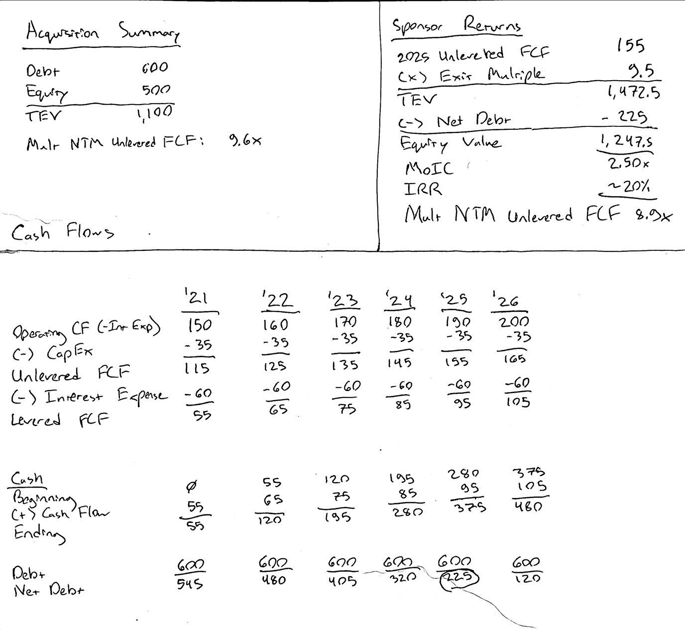
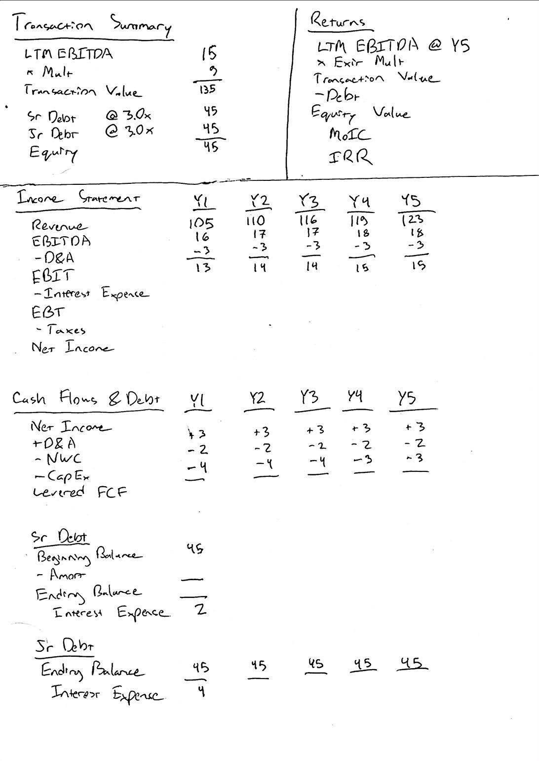
Below is a picture of our pen-and-paper solution, and attached is the Excel version (in case you can’t read our handwriting).

  1. The company’s net debt at exit (2025) is 225.
  2. The company’s equity value at exit is 1,248. The sponsor’s MoIC is 2.50x, and the sponsor’s IRR is 20%.
  3. Asking to compare the entry and exit multiples is somewhat of a trick question. Since you don’t know the company’s 2020 financials, you can only calculate a forward entry multiple. That’s why we added an extra year of cash flows in our solution (above). We need the 2026 cash flows in order to derive the forward multiple at exit, so that we can compare the entry and exit multiples on an apples-to-apples basis (+ 5 points for banker jargon). The forward entry multiple is 9.6x (EV / NTM unlevered FCF). The forward exit multiple is 8.9x; therefore, this investment scenario projects multiple contraction. Usually, you would prefer to see multiple expansion, but the fact that the sponsor achieves a 20% IRR anyways is indicative of strong cash flows.

Step-by-Step Guide

1) Set up your template

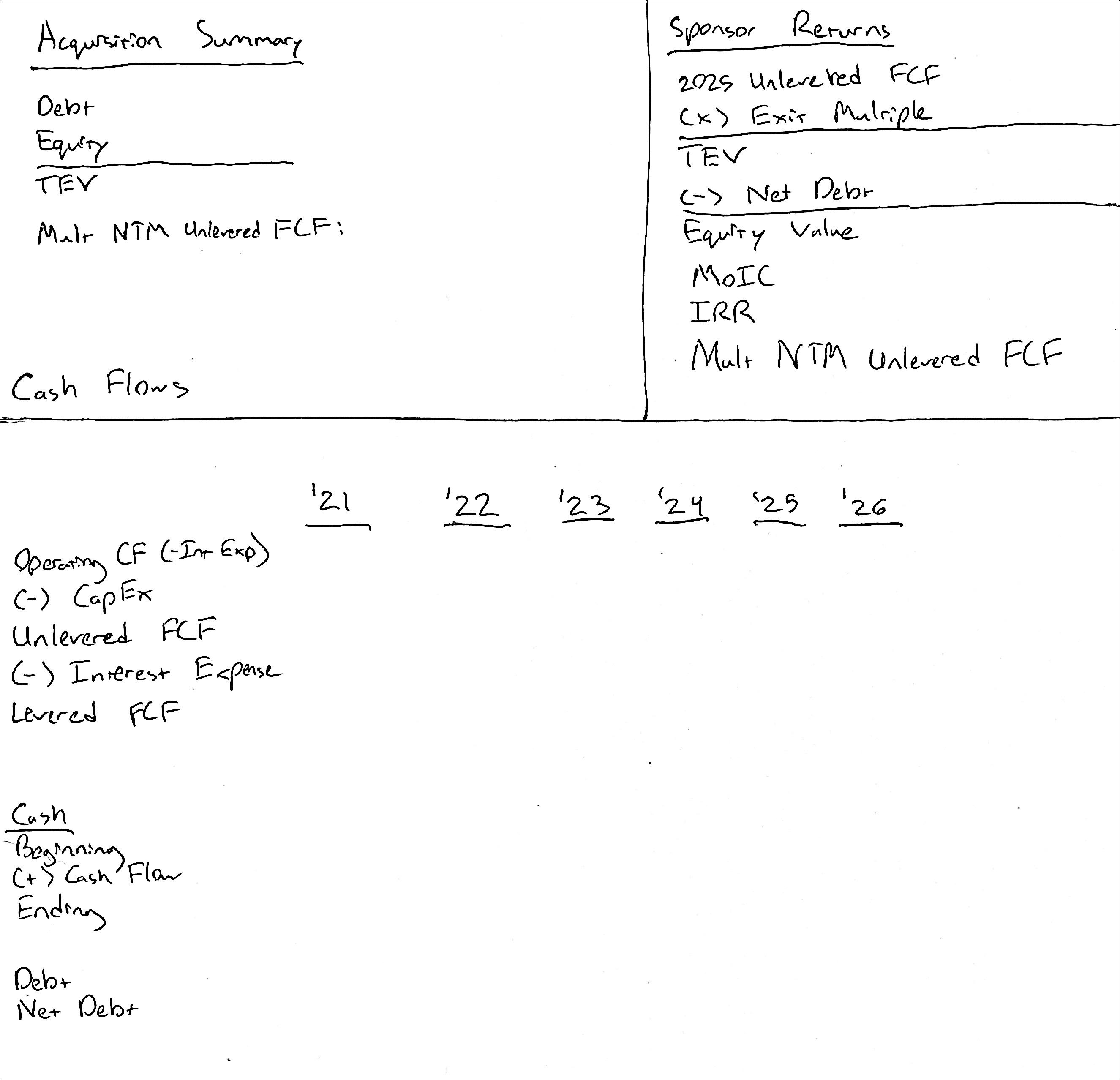
Below is an image of the template we’re using. You’ll notice we have three basic sections:

  • Acquisition Summary
  • Sponsor Returns
  • Cash Flows

Since we’re given the cash flows in the assumptions, we don’t need an income statement.

Also, while it may feel awkward to use free cash flow for calculating multiples, as opposed to EBITDA, remember that’s what EBITDA is supposed to be a proxy for: unlevered FCF.

2) Fill out acquisition summary

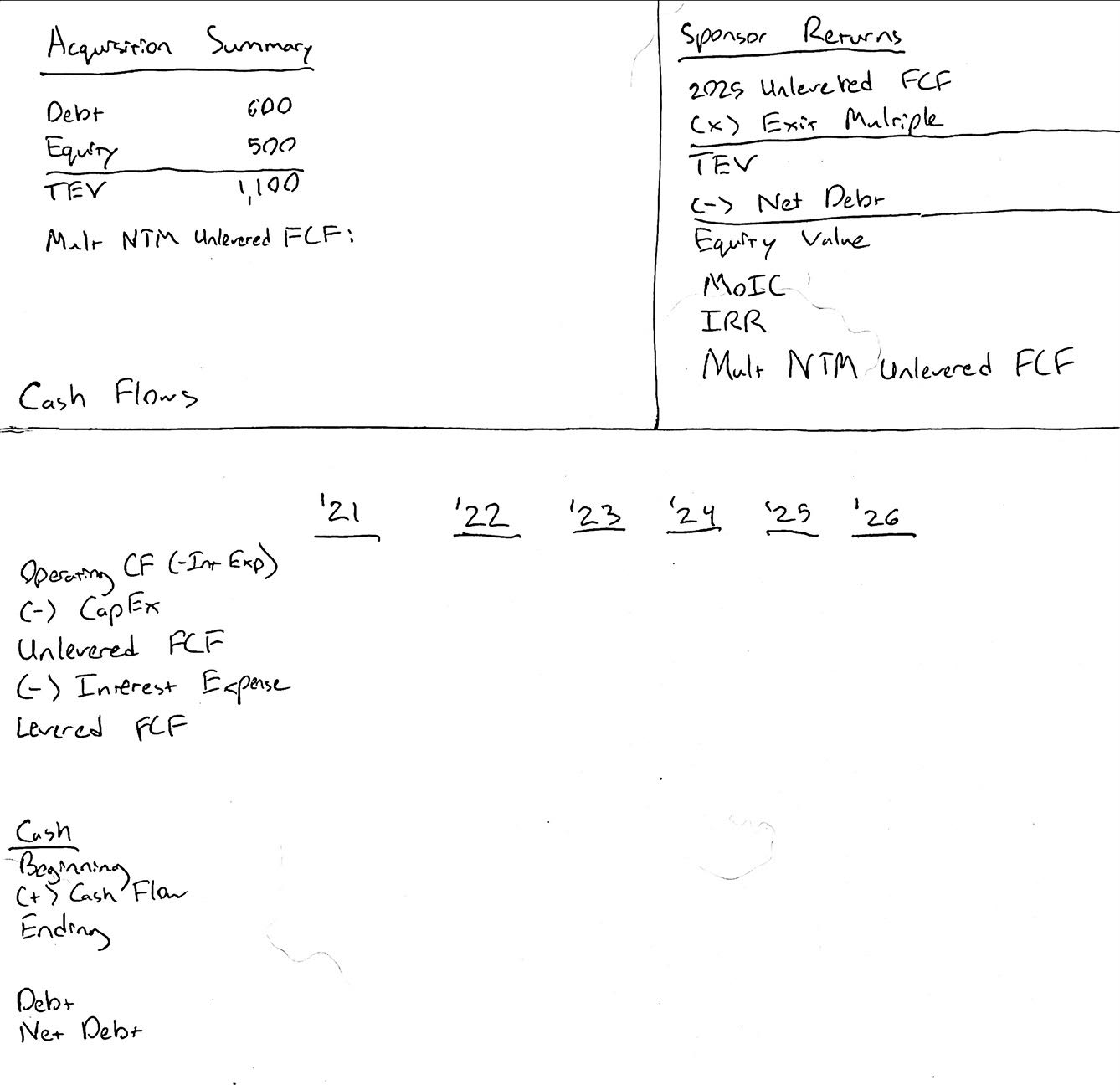
We can fill out the acquisition summary using the provided assumptions. Below is our updated template:
We left the NTM entry multiple blank for now.

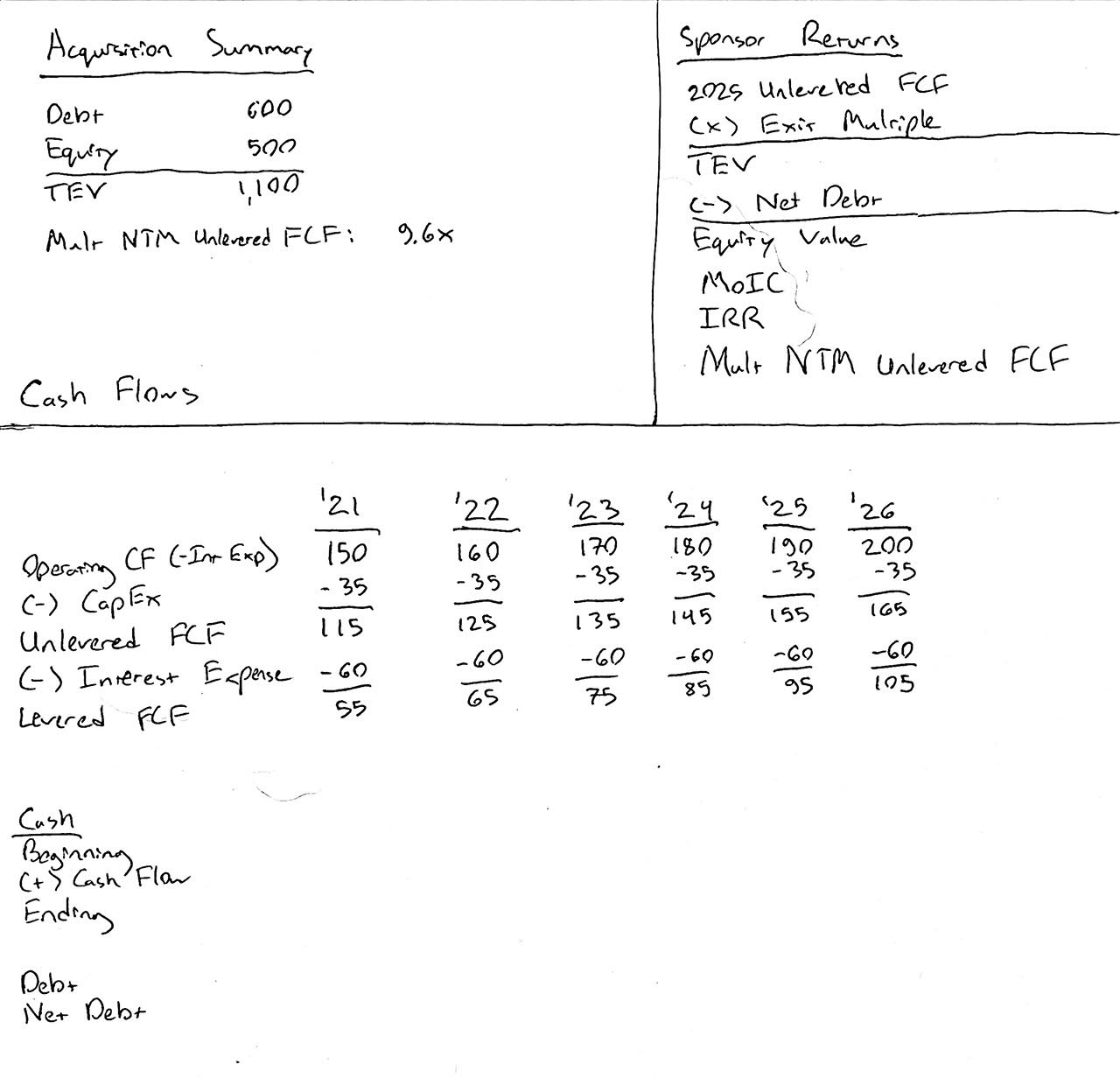
3) Fill out the cash flows

Next we calculate the cash flows. We’re given the 2021 operating cash flow (excluding interest expense), and we’re told the value increases by 10 each year. CapEx is held constant at 35 annually.

Cash Flows Refresher
Levered Free Cash Flow = Cash Flow from Operations - CapEx.

We call it “levered” free cash flow, because cash flow from operations is calculated starting with net income, which includes the impact of interest expense. Therefore, levered free cash flow includes the impact of financial leverage.

Unlevered Free Cash Flow = Levered FCF + Interest Expense - Interest Expense Tax Shield.
Unlevered Free Cash Flow = Cash Flow from Operations (excl. Interest Expense) - CapEx

Rather than paying down debt each year, we’re building a cash balance. Therefore, we can use the same interest expense each year (10% x 600 debt = 60).

We can also add the missing multiple in our acquisition summary (using the 2021 unlevered free cash flow).

4) Calculate net debt

This should be straightforward. The debt balance doesn’t change, and cash increases each year.

Below is our updated template:

5) Calculate sponsor returns

The sponsor sells the company after 5 years - at the end of 2025. We calculate the transaction value using an LTM unlevered FCF multiple (9.5x per the assumptions).

Then, we subtract net debt to derive the sponsor equity value.

Sponsor Returns
Whenever you are asked to calculate a sponsor’s returns, you should include both the MoIC and the IRR. If you’re unsure why you should include both, or if you’re a little fuzzy on sponsor returns, check out our intermediate LBO tutorial for a more in-depth discussion.

The MoIC, or Multiple of Invested Capital, compares the cash earned to the cash invested.

MoIC = Cash sponsor receives / Sponsor equity investment

Remember: a shortcut for calculating the IRR uses the MoIC:

IRR = MoIC ^ (1 / years of investment) - 1

But this shortcut only works when there’s a single investment cash flow (i.e., the sponsor didn’t invest more money later on) and a single exit cash flow (i.e., a clean sale with no dividend recaps or earnouts).

Comparing Multiples
One of the questions above asked us to compare the entry and exit multiples. This was a bit of a trick question, because we can only calculate a forward multiple for the initial transaction. Therefore, we need to add an extra year of cash flows (2026), so that we can calculate an implied forward multiple at exit and properly compare the two. Dividing the exit transaction value by our 2026 unlevered free cash flow, we get an implied forward multiple of 8.9x. Therefore, this investment scenario is showing modest multiple contraction, since the forward multiple at exit is less than the initial forward multiple.

Below is our completed template:

Next Steps

Nice job working through this tutorial!

If you’re preparing for private equity interviews, you should practice this problem weekly until you can complete it in less than 5 minutes. Also, make sure you understand the concepts it’s testing:

  • Levered vs. unlevered FCF
  • Sponsor returns calculations (MoIC, IRR, etc.)
  • Comparing multiples on an apples-to-apples basis (forward multiples shouldn’t be compared to LTM multiples)
  • Multiple expansion

Check out some of our other tutorials (all free):

  1. Easy LBO Guide
  2. Intermediate LBO Guide
  3. Advanced LBO Guide
  4. Ability-To-Pay Analysis
  5. Private Equity Modeling Course

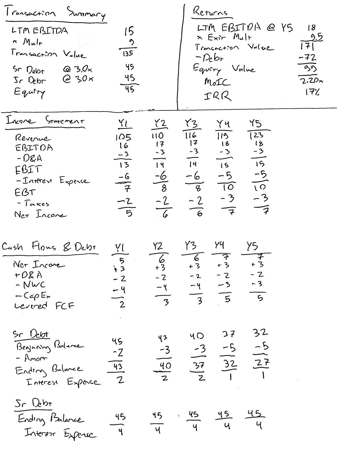
Paper LBO - Step-by-Step Example

Introduction

The dreaded paper LBO is a common obstacle during the private equity recruiting process.

Paper LBOs can be intimidating, in part, because they’re not something you do as a banker or a consultant. Maybe you make real LBOs, which are good preparation for private equity modeling tests, but paper LBOs are a different beast.

The What

First, what is a paper LBO?

A paper LBO is a simplified LBO that can be completed with pen and paper quickly (ten minutes tops).

The Why

Why does anyone bother with paper LBOs? What’s the point?

Paper LBOs are used during private equity interviews to test the following:

  1. That you understand LBO mechanics well enough to perform the calculations with pen and paper – not using a well-trodden Excel template that has been passed down through generations of banking analysts
  2. That you can do simple math quickly while under pressure - PE folks seem to think this is important ¯\(ツ)

Paper LBOs demonstrate that candidates can do private equity math on the spot, without Excel. Think back to the good ol’ days. Today’s titans of private equity didn’t even have Excel when they got started. They did some basic spreadsheet math, sure, but it wasn’t the complex analysis that you see today. The upper levels of private equity require suave professionals, who can do basic analysis in their head (or using an iPhone calculator) while golfing several beers deep. That’s a caricature, but you get the point.

So now we know what paper LBOs are and why folks bother. Let’s do one together.

Paper LBO

Calculate the sponsor’s IRR and Multiple of Invested Capital (MoIC) using the information provided below:

Transaction Assumptions

  • 9.0x transaction multiple
  • Cash-free, debt-free transaction
  • 3.0x senior secured debt (4% interest rate, repayable immediately)
  • 3.0x junior debt (8% interest rate, no early repayment)
  • No transaction expenses

LTM Financials

  • 100mm Revenue
  • 15mm EBITDA

Projections

  • 5% sales growth Y1 - Y3, followed by 3% sales growth
  • Constant EBITDA margin
  • 4mm CapEx Y1 - Y3, then 3mm CapEx per year
  • 3mm depreciation & amortization (D&A) each year
  • 2mm increase in net working capital (NWC) each year
  • 30% tax rate

Exit Assumptions

  • Exit after 5 years at 9.5x LTM EBITDA
  • Cash-free, debt-free transaction
  • No transaction expenses

Simplifying Assumptions

  • Round all values to whole numbers (in millions). For example, if you calculate EBITDA using revenue (110mm) and the EBITDA margin (15%), the precise value is 16.5mm, but you can round it to 17mm. Adding decimal places is tedious and doesn’t demonstrate your understanding of LBO mechanics.
  • Calculate interest expense based on the debt balance at the beginning of the given year.

Try It Out

Below, we have the completed version along with a step-by-step guide. Before scrolling further, try building the paper LBO yourself. You should be able to complete it within 10 minutes. If it takes a little longer, that’s okay. Practice makes perfect.

Completed Version

Here’s what our completed version looks like:

We calculated the following sponsor returns:

  • 2.20x MoIC
  • 17% IRR

If you can’t read our handwriting, here’s the completed version in Excel.

Step-by-Step Guide

1. Sketch It Out

This should feel somewhat familiar. Design your template on a sheet of paper. You’ll need the usual LBO sections:

  • Transaction Summary
  • Income Statement
  • Cash Flow Statement
  • Debt Schedule
  • Returns Summary

Here’s what your “paper template” should look like:

2. Basic Financials

  • Let’s fill out revenue, EBITDA, D&A, CapEx and change in NWC using our assumptions.
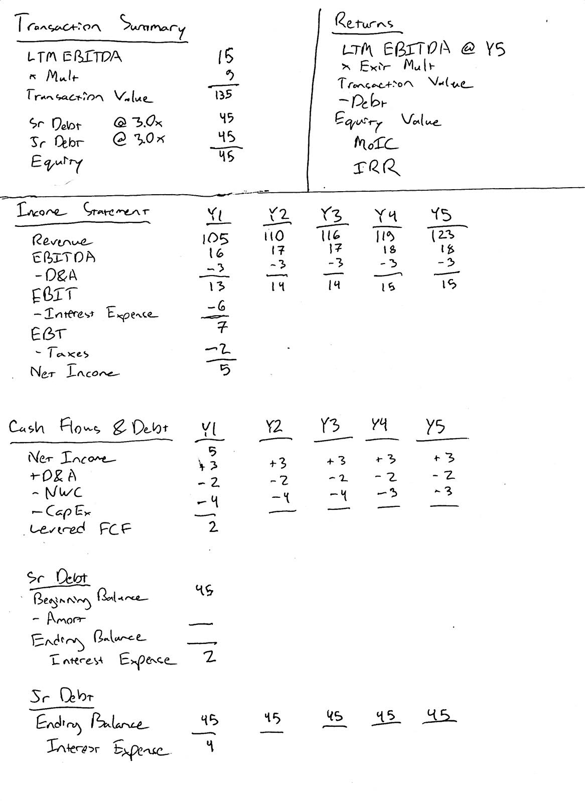
  • D&A, CapEx and change in NWC are provided constants, so we only need to calculate revenue and EBITDA.
  • The revenue values should be: 105, 110, 116, 119, 123
  • The EBITDA values should be: 16, 17, 17, 18, 18

Remember: We’re rounding to whole numbers to make the calculations easier.

Here’s what our paper LBO looks like after this stage:

3. Transaction Summary

Now let’s fill out the transaction summary.

  • We know the transaction multiple and LTM EBITDA, so it’s easy to get the transaction value.
  • Likewise, we know the LBO is financed with 3.0x senior debt and 3.0x junior debt. The remaining funds are provided by the sponsor (the private equity fund).

Here’s what the completed transaction summary looks like:

4. Debt Schedule

In order to complete the income statement and the statement of cash flows, we need to calculate interest expense. Therefore, we need to begin filling out the debt schedule.

  • We’re not paying down any of the junior debt, so the initial 45mm of junior debt will be held constant.
  • We will, however, be paying down the senior debt.
  • Since we’re calculating interest expense using the beginning debt balances each year, there’s no circularity. We can perform all of the calculations manually.

Let’s calculate the interest expense for year 1. We have 45mm of senior debt @ 4% and 45mm of junior debt @ 8%. Senior debt interest expense is 2mm (remember - rounding to whole numbers) and junior debt interest expense is 4mm.

Here’s what your paper LBO should look like so far:

5. Y1 Cash Flows

Since we have the Y1 interest expense (6mm total), we can complete the income statement and cash flows for Y1.

Here’s what your LBO should look like after this step:

6. Y1 Debt Paydown

Now that we’ve calculated the levered free cash flow (FCF) for Y1, we can calculate the senior debt amortization and ending balance.

We should pay down as much debt as possible, using all available cash flow (2mm). Therefore, our ending senior debt balance for Y1 is 43mm. And likewise, the beginning senior debt balance for Y2 is 43mm.

Here’s what your LBO should look like after this step:

7. Y2 - Y5 Interest Expense, Cash Flows & Debt Paydown

We’ve calculated the interest expense, levered FCF and debt paydown for Y1. Let’s fill out the remaining years following this pattern.

Here’s what your LBO should look like after this step:

8. Returns Summary

At this point, calculating the sponsor returns should be straightforward.

  • Y5 LTM EBITDA is 18mm. The transaction value = LTM EBITDA (18mm) x 9.5 = 171mm.
  • We have 72mm remaining debt (27mm senior debt + 45mm junior debt).
  • Therefore, the sponsor equity value = 99mm, yielding a MoIC of 2.20x and a 17% IRR.

Here’s the completed paper LBO:

Bonus Question

You may have noticed that the returns above benefited from multiple expansion.

What would the sponsor returns have been without multiple expansion?

  • Transaction Value = 18mm x 9 = 162mm.
  • Equity Value = Transaction Value (162mm) - Debt (72mm) = 90mm
  • MoIC = Equity Value (90mm) / Sponsor Equity (45mm) = 2.00x
  • IRR = 15%

Final Thoughts

Again, practice makes perfect. Once you can fly through this example under 10 minutes, you will be well prepared for any paper LBO. Sometimes interviewers include more manual calculations (e.g., D&A as percentage of revenue), but that should not increase the difficulty of the exercise. Most paper LBO exercises that you encounter will be simpler than this one.

Next Steps

To learn more, check out our comprehensive (and free) private equity modeling course.

Also, here’s another practice paper LBO based on a real modeling test.

Advanced LBO Modeling (Part 1)

Intro

This article is a continuation of our private equity modeling series. We’re going to show you how to take our intermediate LBO template and turn it into a more advanced, flexible LBO model.

There’s a lot of material to cover, so we’re going to split this tutorial into a series of posts. This one will show you how to integrate casing, flexible financing assumptions, and sensitivity analysis. Future posts will cover topics including operating models and add-on acquisitions.
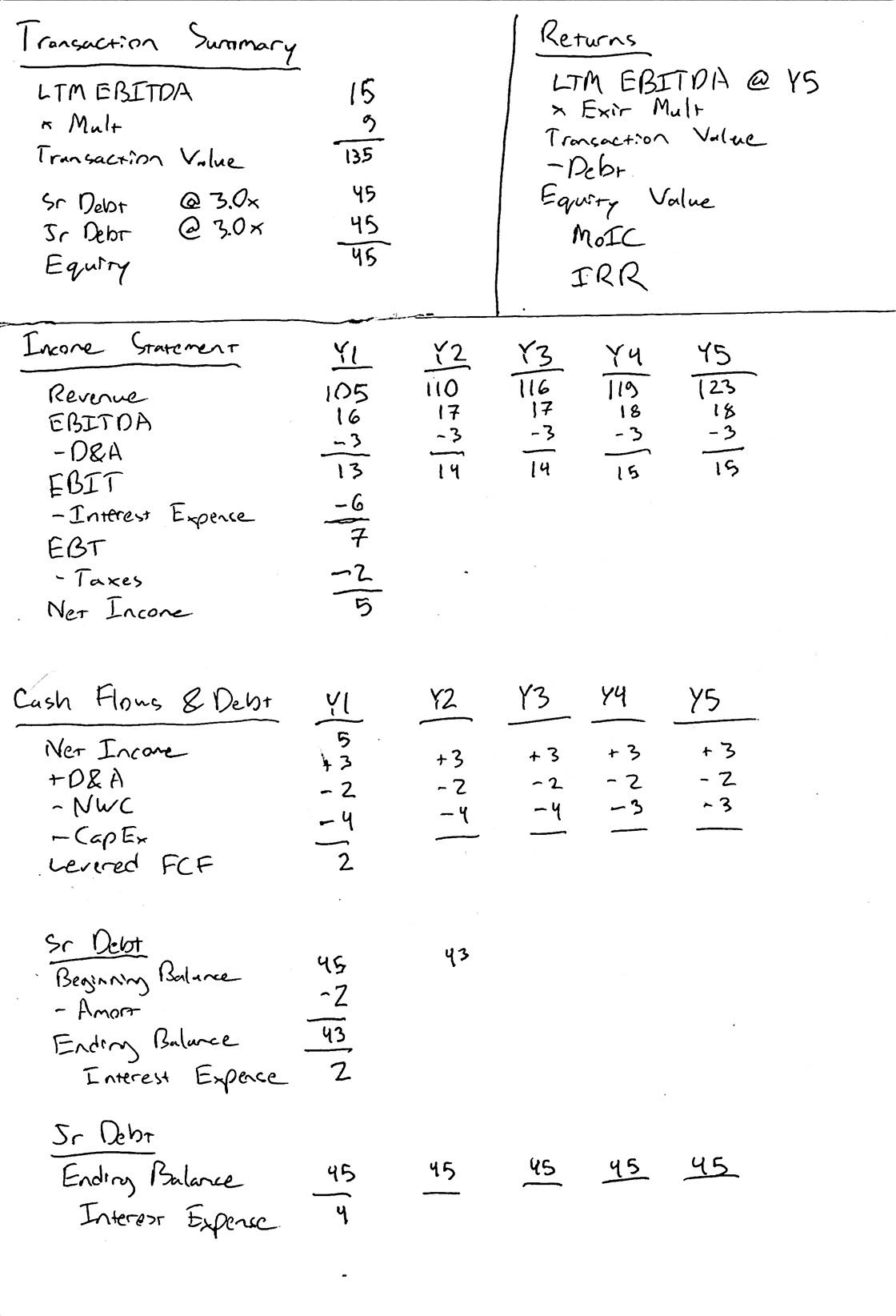
We highly recommend completing the following tutorials before proceeding with this one:

  1. Intermediate LBO Modeling
  2. Ability-to-pay Analysis
  3. Value Creation Analysis
  4. LBO Equity Waterfall
  5. Adding Flexible Cases to a Financial Model
  6. Excel Data Tables, the Right Way

Goal

By the end of this tutorial, you’ll know how to build a sophisticated, flexible LBO model.

Starting Point

As a starting point, we’ll use the completed LBO model from our LBO equity waterfall tutorial.

Download the template, and let’s take a look.

You’ll notice the model includes the following four tabs:

  1. ATP - this is our ability-to-pay analysis
  2. Contrib - this is our basic value creation analysis
  3. LBO - this is our intermediate LBO model
  4. Equity Waterfall - this is an illustrative equity waterfall

Of these, we’re going to focus almost entirely on the LBO tab. The other three tabs are supplemental analyses, but we’re including them here for the reasons listed below:

  • ATP - I include an ability-to-pay analysis with any LBO model. The ability-to-pay analysis is easy to add, and it’s a great sanity check for the LBO.
  • Contrib - Likewise, I always include a value creation bridge. It’s important to understand what’s driving the modeled returns.
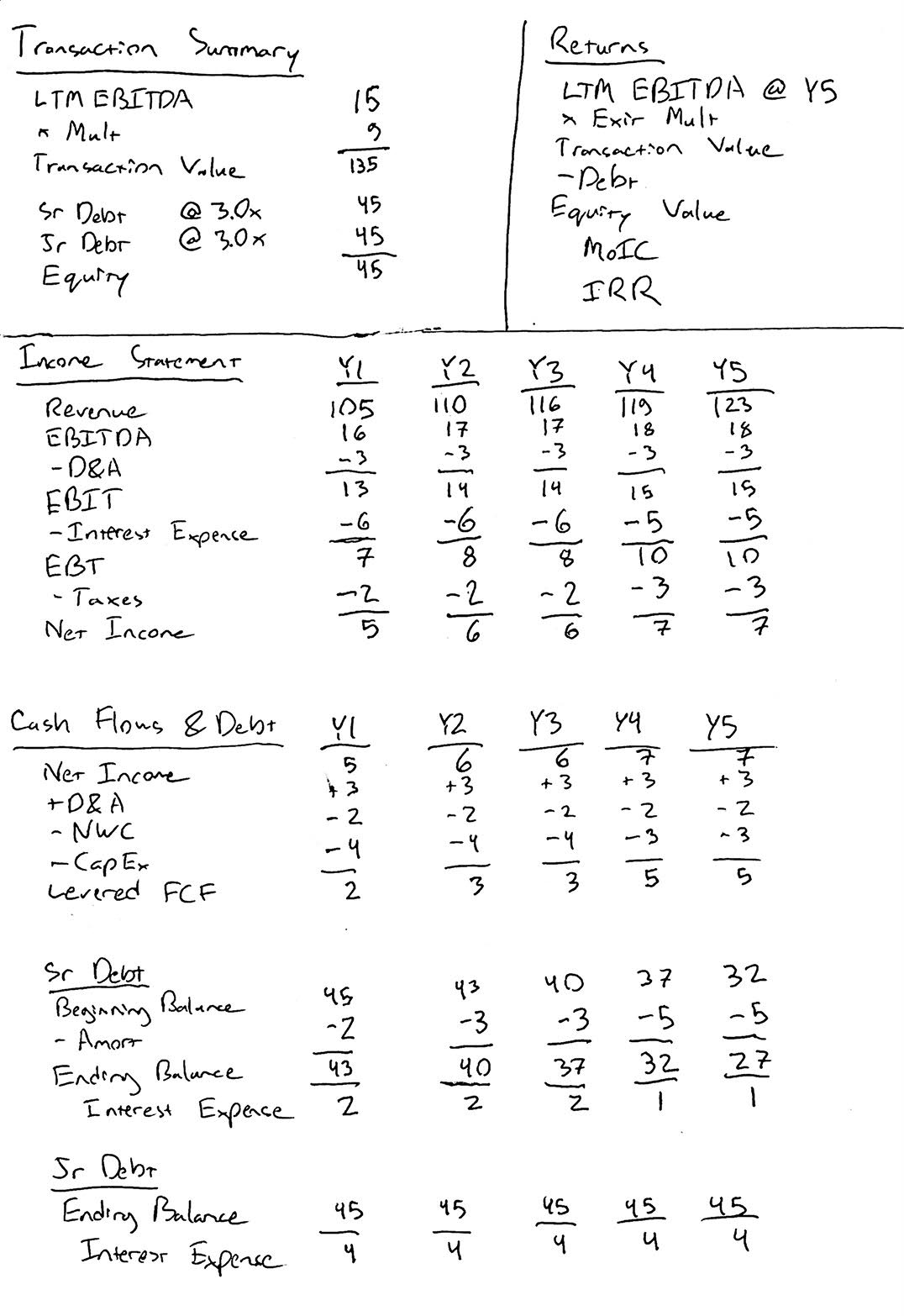
  • Equity Waterfall - This is not relevant in banking, but will be present in any serious private equity deal.

Let’s get started.

1. Financing Cases

In this first step, we’re going to add flexible financing cases to our model. Right now, the financing assumptions are hard-coded at the top of the LBO tab.

First, some general cleanup:

  • Let’s move the LBO tab to the far left (out of the four tabs).
  • Likewise, since we’ll be adding more tabs to the model, let’s color code the tabs. Make the LBO tab dark blue, and you can make the other tabs all another color.
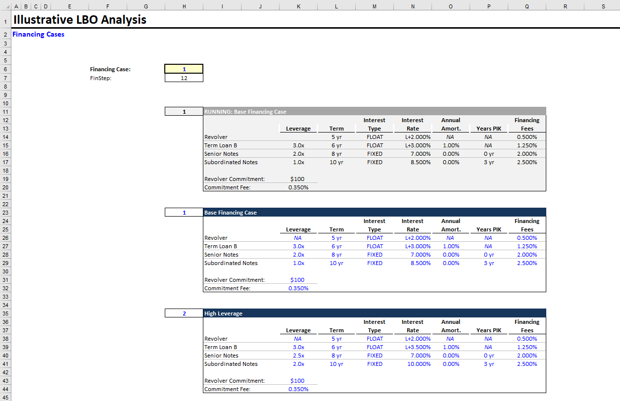
Now, for the main course.

  1. Create a new tab called FINCASE.

    Shortcut for creating a new tab: Shift F11
    Shortcut for renaming a tab: ALT + H + O + R

  2. Now, let’s go to the LBO tab and copy the entire financing assumptions table (located at the top of the tab). We’re copying it so that the sensitized assumptions match the LBO format perfectly.

  3. Paste the copied table at the top of the new FINCASE tab starting at cell I11. The copied table should take up 10 rows, including the blue header bar and the revolver commitment fee.

  4. Skip two rows and paste the table again (in line with the table above). Do this two more times. You should now have four copies of the table, with two rows of spacing after each table. The first copied table will be our output, and the remaining three tables will be our financing cases.

  5. We’ll ignore the first table (the output) for now.

  6. Let’s create our Base Financing Case in the second table. First, change the blue header bar to read Base Financing Case. Also, let’s reduce the Senior Notes to 2.0x Leverage (giving us 6.0x total leverage).

  7. We’ll create our High Leverage case in the third table. Let’s increase the Subordinated Notes to 2.0x Leverage (giving us 7.5x total leverage). Likewise, let’s set the Term Loan B interest rate at L+3.500%, and let’s increase the interest rate for the Subordinates Notes to 10.000%.

  8. In the final table, let’s add our Low Leverage case. We’ll set the Senior Notes to 1.5x leverage, and we’ll set the Subordinated Notes to 0.0x leverage (no Subordinated Notes). We can also decrease the interest rates, since we have less leverage (L+2.750% for the Term Loan B and 6.000% for the Senior Notes).

    Financing Assumptions
    Remember: These are illustrative assumptions. You should rely on your capital markets team for up-to-date financing assumptions.

  9. Finally, in cell H6 on the FINCASE tab, create a case cell (a thick-bordered cell with a hard-coded number). This is the FinCase cell, which determines the running financing case. You’ll see how it’s used shortly.

  10. Directly below the FinCase cell, calculate the total row height of each financing table (we call this the FinStep).

    FinStep
    Make the formula for cell H7 = ROW(High Leverage Header) - ROW(Base Financing Case Header).

    The Excel ROW function returns the row number for a given cell, so here we’re calculating the total number of rows (including spacing) required for each table.

  11. Formatting: Let’s return to the first financing table (which we referred to as our output). Go ahead and shade the entire table light gray (background color), and make the header bar dark gray. Likewise, change the table font color to black to signify a calculated value (instead of a hard-coded assumption).

  12. Go to the first numerical cell in the output table (revolver leverage - it should read NA), and use the following formula:

    = OFFSET(this cell, H6 * H7, 0, 1, 1)

    (in English)
    = OFFSET(this cell, FinCase x FinStep, 0, 1, 1)

    FinCase tells us which financing case should be running, and FinStep tells us the required number of rows per table.

    Offset Function
    If you’re not confident in your understanding of the OFFSET function, please pause this tutorial and Google it. It’s worth 5 minutes of your time. It might be the most powerful Excel function.

We calculated the FinStep (instead of hard-coding it) using the ROW function, so that if we change the number of rows in our financing assumptions, these functions auto-adjust.

  1. Copy this offset formula (but locking the FinCase and FinStep cells) and apply it to all cells in the output financing assumptions table.

  2. Now when you change the FinCase cell (e.g., set the value to 2), the output table should update auto-magically.

Here’s what your completed FINCASE tab should look like:

Last Step
Return to the LBO tab, and link the Financing Assumptions table to the output table at the top of the FINCASE tab. (Remember to change the font color to green to represent a value linked from another tab.) Now when you change the financing case on the FINCASE tab, it updates the LBO tab as well.

Take a second and think about how powerful this is. You can now add as many financing cases as your hyperactive MD could ever desire, and you can update which case is flowing through your LBO model by changing one cell.

Here’s the completed Excel file for this step. Take a look if you’re stuck or want to verify your work.

2. Master Case Tab

In the prior step, we added casing to our financing assumptions. This made our LBO model much more flexible, but that’s not the end of this story.

There are several other variables we want to sensitize that are independent of our financing assumptions (for example, the transaction multiple). How can we sensitive these other variables along with our financing assumptions?

Here, we rely on the concept of a Master Case tab, which is exactly what it sounds like. It’s a tab that rules all the other case tabs and specifies what the running assumptions are. You may be wondering: Why bother putting the financing assumptions in their own tab? And the answer is: Because we generally think about financing assumptions as a single unit:

Analyst: “Yes, this output is based on our conservative financing case.”
VP: “Well, run the aggressive financing case instead and reprint.”

Similarly, we would separate operating model variables into an Operating Cases tab, also controlled by the Master Case tab.

Below is what our completed Master Case tab will look like:

Now let’s build it. Note: This section draws heavily on our Adding Flexible Cases to a Financial Model tutorial, so give that another read if you’re confused.

  1. Create a new tab (named MCASE).

  2. Let’s list the variables we want to include:

  • Transaction Multiple (EV / LTM EBITDA) and Transaction Value
  • Transaction Expenses
  • Management Rollover %
  • Financing Case (which financing case is running)

    Exit Multiple
    We don’t need to include the exit multiple here, because the LBO tab already sensitizes the exit multiple.

  1. Let’s add the columns. There should be 1 column for each of the variables listed above. I also like to number each case, so the columns should be:
  • Case Number (e.g., 1, 2, 3, 4, etc.)
  • EV / LTM EBITDA
  • Transaction Value
  • Transaction Expenses
  • Management Rollover %
  • Financing Case

    Why include both the Transaction Multiple and Transaction Value?
    An astute reader might wonder why we’re including both the Transaction Multiple and the Transaction Value in our MCASE tab. After all, doesn’t one determine the other?

    Yes, that is true. But we include both, because you want to be able to frame the question either way. For example, you might ask “What does a 925mm deal look like?” or “How do the returns look assuming a 10x transaction multiple?” Sure, you could back out the transaction multiple to get to 925mm, but 10.278x looks rather nonsensical. It will make more sense to someone else, looking at your model, to see 925mm hardcoded directly on the cases tab.

  1. Now, let’s make our first five cases. Across these cases, only the transaction multiple (and therefore, transaction value) will vary; we’ll hold everything else constant. Let’s start the multiple at 8.0x and increase it by 0.5x with each case, so the transaction multiple will range from 8.0x - 10.0x. For the other variables, we can use the existing values hard-coded on the LBO tab (15mm for transaction expenses and 5.0% for the management rollover). We’ll also set the financing case equal to 1 (our base case). Since only the transaction multiples / transaction values differ, we can hard-code these other variables in the first case (blue font for hard-coded values) and we can set the other rows equal to the preceding row (black font for formulas).

  2. Let’s create the Running Case row. Shade the row directly above your new cases medium gray. Likewise, make the font bold and black (for calculated values). In the column where you list case numbers, format the running row cell as a case cell (thick borders, different shading, and blue font).

  3. Name this cell MCASE.

    Naming Excel Cells
    You can name Excel cells following the steps below:

  4. CNTL + F3

  5. New

  6. Enter Name and Press “OK”

    When you name a cell, you can reference that cell using its name in other formulas. For example, we’ll be able to refer to the MCASE cell using its name (e.g., if(MCASE = 1, ...).

    Warning
    Many analysts have a tendency to go overboard with Excel naming. It is best practice to limit the number of named cells in your model.

  7. We want the values in the Running Case row to equal the specified case (the case number in the MCASE cell). Can you figure out how to do this using the OFFSET function? This should feel familiar after the FINCASE tab.

    Answer
    Each cell in the Running Case row = OFFSET(the given cell, MCASE, 0, 1, 1). This just grabs the value from the specified case.

  8. Now create the remaining ten cases shown in the picture of our completed MCASE tab (above). You’ll notice that cases 6 - 10 match the first five cases, except for the specified Financing Case, and that cases 11 - 15 also follow this pattern.

  9. Now your MCASE tab is essentially complete. Make any formatting changes in order to match the image above.

    Remember: Financial models are, in part, communication tools. They’re a way to examine specific scenarios and share your work with others. Clean formatting is a key part of that.

Here’s the completed Excel file for this step.

3. Connect the LBO & MCASE Tabs

This step is quick. We’re going to connect the MCASE tab with the rest of the model. Once it’s connected, by changing the running case number on the MCASE tab, we update our entire model.

Here are the variables we need to link:

  • Transaction Multiple
  • Transaction Expenses
  • Management Rollover %
  • Financing Case

Note: We’re intentionally excluding the transaction value, because it’s already calculated on the LBO tab. I know, I know. We made a big deal about including both the transaction value and the transaction multiple on the MCASE tab, and now we’re only linking one of the values? We included both on the MCASE tab, because we want our cases to be easy to understand. But we only need to link the transaction multiple, because we already calculate the transaction value on the LBO tab. Make sense?

First, let’s link the transaction multiple, transaction expenses, and management rollover percentage on the LBO tab. These assumptions are all hard-coded at the top of the model. Simply replace the hard-coded values with links to the correct cells in the MCASE running row. Remember to change the font colors to green (green signifies a value linked from a different tab).

Last, let’s link up the financing case. Go to the FINCASE tab and set the Financing Case cell equal to the running financing case on the MCASE tab. The Master case tab rules all other casing. It provides a single control panel for your entire model.

Here’s the fully linked Excel file if you want to check your work.

4. LBO Cleanup

This is another quickie. We’re going to make a couple minor changes to the LBO to prepare for the next step.

  1. Right now, the exit multiples in the LBO returns calculations vary based on the running transaction multiple. We don’t want that anymore. Instead, we want a fixed range of exit multiples.

On the LBO tab, go to the Illustrative Returns section at the bottom of the tab. Hard-code the first transaction multiple in the enterprise value calculations; set it to 7.0x. For the multiple below that, set it to the preceding value + 0.5. Copy this formula down for all the remaining multiples. You should now see transaction multiples ranging from 7.0x to 11.0x in increments of 0.5x.

  1. Next, let’s put boxes around the returns metrics we’ll use for our sensitivity analysis (next step). Highlight cells N346:N350 (MoIC), and add a border. Do the same for cells N360:N364 (IRR). This serves two purposes:
  • Outlining the values will ensure we don’t link to the wrong column (been there, done that)
  • Makes it easy to spot check our sensitivity tables in the future

Here’s the updated Excel file.

5. Sensitivity Analysis

This section will walk through adding sensitivity analysis to your model. It draws heavily from our Excel Data Tables, the Right Way tutorial, so if you’re stuck, please reread that article. Long story short: For any sophisticated model, Excel data tables aren’t going to cut it. You need to construct your models with proper casing and sensitivity analysis.

We’re going to make three sets of sensitivity outputs - one for each financing case. Each output will consist of a MoIC (Multiple of Invested Capital) sensitivity table and an IRR sensitivity table. These tables will show our returns metrics at varying entry and exit multiples. Here’s what one of the sensitivity outputs will look like:

Before building the sensitivity output, let’s talk about the various elements in the image above. First, there are the case numbers in the yellow-shaded row. Each column in the output tables is tied to a case number, which refers to a specific case on our MCASE tab. On the right, we see gray-shaded linked values. These are links to the currently running returns metrics on the LBO tab. We also link to the current transaction multiple. Lastly, the values in the sensitivity tables are calculated using the case numbers, these linked values, and the running MCASE.

Enough chitchat. Let’s make some sensitivity outputs.

  1. Create a new tab, and name it Sensitivity.

  2. Add headers and basic formatting to conform to the image above.

  3. Let’s add the case numbers. Each row in the sensitivity tables represents a particular exit multiple (EV / LTM EBITDA). Each column represents an entry multiple (the transaction multiple). We’re fortunate that our LBO tab already sensitizes the exit multiple. Therefore, we can represent each column with a single case (we only need to sensitize the transaction multiple).

The image above shows our entry multiple ranging from 8.0x - 10.0x (same as the exit multiple), which corresponds perfectly to each group of five cases on the MCASE tab. Our first sensitivity output will be for our Base Financing Case, so we’ll use the first five cases (1, 2, 3, 4, 5) here. Fill in the case numbers.

  1. Next, let’s fill in the gray-shaded linked values. The first cell to link is the transaction multiple. You can set it equal to the running transaction multiple at the top of the LBO tab. Then, the next five linked values are the 5-year MoIC values that we outlined at the bottom on the LBO tab.

For the IRR sensitivity table, we can link the entry multiple to the value above (on the Sensitivity tab). We shouldn’t link to the transaction multiple on the LBO tab again, because we’ve already imported that value. The next five values to link are the 5-year IRR values that we outlined on the LBO tab.

  1. Last, we’ll create the formulas for our sensitivity tables. We’ll use self-referencing if statements (as described in Excel Data Tables, the Right Way). If you’re not sure what these are, or how they work in the context of sensitivity tables, go back and reread that tutorial. This is a key concept.

You’ll use the following formula for each cell in the data table (including the entry multiple column headers):

= if(MCASE = case number row, linked value column, self)

Make sure to lock the row, for the case number, and the column, for the linked value. This formula ensures that a column only updates when the specified case is running.

You’ll notice that your sensitivity tables have the same values in every column (including the entry multiple column headers). That’s normal! You haven’t run all the cases yet.

  1. Now we’ll replicate the sensitivity output for our two remaining financing cases.
  • First, copy the rows containing both sensitivity tables.
  • Then, paste the copied rows beneath the prior output.
  • You’ll need to update the case numbers.
  • We’ll use the same gray-shaded linked values, but instead of linking to another tab, link to the imported values above. This way, we’re only importing the running MoIC and IRR values once.
  • Update self-referencing if statements to use the new case numbers.

You should now have three well-built sensitivity outputs, one for each financing case. Here is the completed Excel sheet if you’d like to compare.

6. Running All Cases

We’ve built our sensitivity outputs. Now we need to run all cases, so that our self-referencing if statements update. To do this, we’re going to use the technique we introduced in our Excel Data Tables, the Right Way tutorial:

  1. Go to the MCASE tab.
  2. To the right of your cases, with a couple extra columns for spacing, copy the row numbers. Then, in the running case row above the case numbers, set the cell equal to the current date and time:

    cell = NOW()

Your MCASE tab should look like this.

  1. Next, we’ll use Excel’s native data table functionality to run all cases:
  • Highlight the case numbers and date
  • Create an Excel data table: ALT + A + W + T
  • Enter MCASE as the column input cell (leave the row input cell blank), and press OK
  1. Press F9 to run all calculations.
  2. Go to the Sensitivity tab, and confirm that your sensitivity outputs have updated.

Here’s the completed Excel file.

7. Final Cleanup

As a best practice, we don’t like to save Excel files with active data tables. Data tables can really slow down Excel, and self-referencing if statements enable anyone opening the file to see the various scenarios and returns.

Therefore, delete the Excel data table from the MCASE tab and resave the file.

Here’s the final version.

Conclusion

Now you know how to add sophisticated casing and sensitivity analysis to your LBO. Reach out with any questions or feedback.

Mid-Year Discounting

Introduction

This post will be a quickie explaining mid-year discounting (a.k.a. mid-year convention). We introduced this concept in our DCF tutorial, but we’re going to fully explore / explain it below.

But why? Who cares?

  • Mid-year discounting is standard practice for investment bankers.
  • Furthermore, by learning about mid-year discounting, you improve your understanding of valuation.

So yeah… it’s important and useful.

Background

Let’s review some background info (bare with me). DCF stands for Discounted Cash Flow analysis. It refers to the common valuation methodology of projecting an asset’s cash flows and then discounting those cash flows to present value. Theoretically, the asset’s value equals the sum of those discounted cash flows. So far so good? If not, this article might not be the right starting place for you.

Remember - each period’s cash flows are discounted by the corresponding time period. For example, let’s assume we’re evaluating RandomCo.

  • Over the next year (T = 1), RandomCo is projected to earn 100mm in cash (CF1).
  • The following year (T = 2), RandomCo is projected to earn 110mm in cash (CF2).
  • The following year (T = 3), RandomCo is projected to earn 120mm in cash (CF3).
  • Etc.

    We can discount those cash flows to present value using the general formula:
    PV = CF / (1 + R) ^ T

    R is the discount rate.

    Now let’s apply that formula to derive the value of RandomCo:
    RandomCo value = CF1 / (1 + R)^1 + CF2 / (1 + R)^2 + CF3 / (1 + R)^3 + …

In this example, we implicitly assume that RandomCo earns its cash at the end of each time period, because we’re discounting each period’s cash flows by the full time period. But in the real world, that’s usually incorrect. Most businesses earn money throughout the year (or month or whatever time period you’re evaluating). By discounting these cash flows by the full time period, we unfairly over-discount the cash flows. Let’s look at RandomCo again:

We know that over the next year (T = 1), RandomCo is projected to earn 100mm in cash. Furthermore, we can assume that RandomCo will be earning 8.5mm of cash each month.

Yet we’re discounting all of that cash as if it were earned at year end. This is unfairly punitive, especially for cash earned in the next few months.

Mid-year Discounting

Enter mid-year discounting (a.k.a. mid-year convention).

Mid-year discounting is a simple correction for this over-discounting phenomenon. Using mid-year discounting, we treat all cash flows as if they occur at the midpoint, rather than the end, of the given time period. But in order to apply mid-year discounting, we must assume an asset’s cash flows are evenly distributed throughout the time period. For companies that have irregular or lumpy cash flows (e.g., highly seasonal businesses), mid-year convention is not a good fit.

Okay, let’s apply this to RandomCo:

RandomCo value = CF1 / (1 + R)^0.5 + CF2 / (1 + R)^1.5 + CF3 / (1 + R)^2.5 + …

We’re subtracting 0.5 from each time period, because we’re applying mid-year convention, and we’re treating the cash flows as if they are earned at the midpoint of each period (mid-year).

Is mid-year convention appropriate here?
Yes, RandomCo is projected to earn an equal amount of cash each month. Therefore, using the period’s midpoint for discounting is reasonable. Roughly half the cash flows will be over-discounted (months before the midpoint), and roughly half the cash flows will be under-discounted (months after the midpoint). The “misses” on both sides cancel each other out.

Mid-year discounting is not perfect, but in many cases, it captures economic reality better than period-end discounting.

A Little More Theory

Most discussions of mid-year discounting skip straight to Excel at this point. But there’s still some gold to extract.

Time Period

First, it’s important to note that mid-year discounting has a bigger valuation impact when the time period is longer. For example, mid-year discounting will have a larger impact on an annual DCF than on a quarterly DCF.

Theoretically, as we shrink the time period (from years… to months… to days), the potential over-discounting (which mid-year convention corrects for) converges to zero. Likewise, the difference between mid-year discounting and period-end discounting also converges to zero. So when we’re evaluating shorter time periods, mid-year discounting has a smaller valuation impact.

Business Model

Most bankers apply mid-year convention by default, and it’s generally a fair assumption: Many businesses earn cash semi-evenly throughout the year.

You should, however, think critically about the given business. How much seasonality does it have? For example, some specialty retailers do the bulk of their business at year end. For companies like these, mid-year convention is inappropriate - and period-end discounting is, in fact, better.

Impact

How much does mid-year convention really matter?

To answer this question, we’re going to return to our DCF template. Our template contains a switch (at the top) to turn on / off mid-year discounting. This switch will allow us to test the valuation impact of mid-year convention.

Our DCF template fully incorporates mid-year discounting, and you can review the template to examine formulas. If you have questions on specific formulas, check out our DCF article, which walks through the trickiest parts. If you still have questions after reading the article, please reach out.

Before getting into the numbers, we have a question to ponder: Under what conditions will mid-year convention have the largest valuation impact?


First off, by “valuation impact” we mean the difference in value between a DCF using period-end discounting and a DCF using mid-year convention.

Longer Time Period = Bigger Impact
We already gave you this one. Mid-year convention has a lower impact when evaluating shorter time periods, and conversely, it has a bigger impact when evaluating longer time periods.

Bigger Discount Rate = Bigger Impact
A higher discount rate will lead to a larger impact. It should be pretty intuitive that the higher the discount rate, the higher the impact of extra discounting.


Now, Some Numbers

Below is a comparison of enterprise values calculated using the perpetuity growth method - with and without mid-year discounting. We calculated these values using our DCF template and an Excel data table (I know, I know - we should have been classier and made our data table the right way).


These enterprise values seem pretty similar, so let’s look at them on a percentage basis:

(Here’s the Excel backup if you’re curious.)

Takeaways

  • A 3 - 6% increase in value is meaningful. For a billion dollar company, that means an extra 30mm - 60mm.
  • Obviously, the details of this particular DCF are contrived, but the impact is real.

Conclusion

You should now fully understand what mid-year convention is and when and why it’s used. If in the future, your VP asks you to apply mid-year discounting to a highly seasonal business, you can politely point out that mid-year discounting might not be appropriate (just kidding - maybe skip that part).

Remember it’s important to think critically about both explicit and implicit valuation assumptions.

Private Equity Modeling Course

Introduction

This post organizes some of our existing content into a self-study course for private equity finance. We wrote the content and the outline below primarily for two groups of people:

  1. Investment banking analysts preparing for private equity (both for interviews and actual associate roles)
  2. Ambitious students looking to prepare for their first finance jobs

In retrospect, our investment banking years prepared (most of) us well for private equity, but we felt varying degrees of anxiety: Have I learned what I need to? Anything I should review? It was hard to get answers, and it’s still difficult now, although perhaps the requirements of the role are a bit more transparent. Regardless, we hope the materials below will help you review and fill any gaps in your education. We believe strongly that educational content should be free and available online.

If you master the concepts below, you will be ready for any private equity associate role.


1) LBO Modeling

LBO modeling is the most fundamental skill for private equity associates. It encompasses several different branches of knowledge:

  • Excel fluency
  • Finance & accounting
  • Capital structure

1.1) LBO Basics

Start with our easy LBO model. Master this template and the contained concepts before advancing.

1.2) Capital Structure Fundamentals

Now that you’ve mastered some LBO basics, let’s explore capital structure from a first principles perspective.

One of the most important takeaways from this article is that sponsor returns are the product of two components:

  1. unlevered asset returns (ROA) and
  2. capital structure.

While you will build skill in structuring transactions and arranging financing, the surest path to success is acquiring the best assets at the cheapest prices (high ROA). If the unlevered return is high, you don’t need a genius capital structure to achieve great equity returns.

1.3) Intermediate LBO

This is the LBO template we used to prepare for private equity interviews. It is more sophisticated than any modeling test you’ll encounter. Furthermore, it’s a good template for any first-pass LBO (e.g., digest this CIM and tell me what you think).

If you can complete this LBO in under two hours (without looking at the instructions), you’ll be ready for any private equity modeling test.


2) LBO Returns

Great, you’ve mastered LBO modeling fundamentals. But what is your LBO really telling you? What’s driving that juicy 25% IRR?

This section will focus on interpreting and thinking critically about LBO models.

2.1) LBO Value Creation

Here, we introduce the dreaded value creation bridge. Whenever you make an LBO, you should understand what is driving your returns. For example, how much (what %) is the debt financing contributing to your returns?

Many value creation bridges are much more complicated than this one. Over the course of a deal, as the sponsor gathers information and refines the operating model, the private equity associate may create a detailed value creation bridge showing the impact of each operational lever. For example, the revenue growth and margin improvement for each division might be included as separate line items. This level of granularity enables you to answer questions, like: How much is division A’s revenue growth contributing to our overall returns? What happens to our returns if division A stagnates?

Some may call this false precision, but doing this exercise forces you to confront all the implicit assumptions in your investment case. Wow, I didn’t expect leverage to contribute so heavily to returns. Or: That add-on acquisition is responsible for 30% of total value creation. That seems iffy.

This is a really important concept, so take your time working through this template. It may seem deceptively simple.

2.2) Understanding Multiple Expansion

Multiple expansion is a fundamental finance concept and impacts LBO returns.

Go back through our intermediate LBO template and see how much multiple expansion affects projected returns.

2.3) Ability-to-Pay

Ability-to-pay analysis is basically a reverse LBO. Rather than starting with the purchase price and calculating implied returns, you start with the required returns and calculate the maximum implied purchase price.

This is primarily a sellside tool, but can be useful in framing bid strategy and in general, for understanding LBO drivers.


3) Advanced LBO Functionality

At this point, you’ve learned LBO modeling and how to analyze LBO returns. This section will introduce advanced LBO modeling concepts.

3.1) Dividend Recaps

Dividend recaps are a way to return capital to shareholders while retaining control of the underlying company. Modeling dividend recaps as part of an LBO can be tricky. The attached Excel template shows you one method for layering additional transactions on top of your base LBO model.

3.2) Equity Waterfall

When creating a simple LBO, you generally group all shareholders into a single line item (“Sponsor Equity”) and calculate aggregate equity returns. But as you progress further along in a deal, you generally outgrow this approach.

The invested equity can be structured into numerous tranches, and when combined with management’s equity-based compensation, the resulting equity structure can be quite complex.

While each equity waterfall is unique, it’s important to understand this concept, because it surprises many ex-bankers. You’re used to thinking about equity as one or two uniform tranches. But the equity split between the sponsor and the management team can be nuanced and is an important negotiation point.

3.3) Casing & Sensitivity Analysis

Adding flexibility and proper casing to your model is key. This guide shows you how to turn our intermediate LBO template into a sophisticated, flexible model.


Appendix A - Other Modeling Topics

This is an assortment of other financial modeling topics that are applicable to private equity.

A-1) Accretion / Dilution

Accretion / (dilution), while primarily relevant to strategics, can be useful in evaluating add-on acquisitions. Furthermore, many sponsor exits are sales to strategics. Understanding how they evaluate transactions is key.

A-2) Adding Cases to Your Model

Over the course of a deal, you’ll be asked to evaluate many different scenarios and potential outcomes. This article lays out a simple example of adding cases to your model.

A-3) Self-Referencing If Statements

Self-referencing if statements are an extremely powerful Excel feature and can be used to make data tables that don’t slow down your model. This is the right way to create data tables.

What Is Multiple Expansion?

Introduction

This is a quickie. Someone asked, and we’re answering.

Actually, this is long overdue given we’ve named the site after multiple expansion.

This post will strive to:

  1. define multiple expansion
  2. explain how the term is relevant to investing, and
  3. walk through a couple examples

Definition

When a buyer sells an asset for a higher multiple than the multiple that the buyer originally paid, that growth in multiple is called multiple expansion.

The inverse could be called multiple contraction, but the term isn’t commonly used, perhaps because no one likes to highlight that they overpaid.

Simple Example

Let’s walk through an example:

Some years ago, private equity firm Pirate Capital bought a shipping business for a total enterprise value of 100. At the time, the business had 10 of LTM EBITDA. Therefore, Pirate Capital paid a 10x TEV / LTM EBITDA multiple.

Now, the business has 12 of LTM EBITDA, and Pirate Capital sells the business for a total enterprise value of 144, which represents a 12x TEV / LTM EBITDA multiple.

Since the exit multiple (12x) is greater than the entry multiple (10x), there was multiple expansion.

Here’s another:

Pirate Capital bought a sailboat business for a total enterprise value of 110. At the time, the business had 10 of LTM EBITDA. Therefore, Pirate Capital paid a 11x TEV / LTM EBITDA multiple.

Several years later, Pirate Capital sold the business for a total enterprise value of 150 when it had 15 of LTM EBITDA.

Since the exit multiple (10x) was less than the entry multiple (11x), there was multiple contraction.

Context

Ok, who cares? The multiple’s bigger, I get it.

Well, it is just jargon, but multiple expansion is in many ways the alchemy of investing. You take the same business, apply a higher multiple to it, and profit. Think about it - hypothetically, even if the business doesn’t grow at all, as long as the exit multiple is higher, the investors make money.

The table below showcases the impact of multiple expansion relative to debt paydown and EBITDA growth in a simple LBO.

Key Assumptions
Initial Investment

  • 100 LTM EBITDA
  • 1,000 TEV (10x TEV / LTM EBITDA)
  • 60% debt / 40% equity

Performance

  • 5-year hold
  • 20% EBITDA growth
  • 40% debt paydown

As you can see, even relatively small changes in the multiple can dramatically impact returns.

Here’s the Excel backup.

And to learn more about the drivers of LBO returns, check out our LBO value creation article.

Word to the wise

When evaluating potential investments, people sometimes mistakenly talk about multiple expansion as an independent variable. Ex: But if we get some multiple expansion, it could be a real winner…

In almost all cases, however, the multiple is highly correlated with the success of the business. Does the company have strong growth prospects? Are its margins attractive? Etc. If the business is doing well, folks are willing to pay a higher price (multiple). Therefore, it is best to consider the exit multiple a highly correlated booster or detractor from returns. If the deal goes well, and the company is more attractive than it was 5 years ago, someone might pay a higher multiple. Yay, multiple expansion! The inverse is also true. But in both of these outcomes, the multiple is not some independent pinwheel of chance. It is highly dependent on the rest of the deal.

Manufacturing Multiple Expansion

So far, we’ve established that

  1. Multiple expansion is desirable and
  2. it’s correlated with the overall deal.

As investors, how can we manufacture multiple expansion, or ensure that our deals sell for higher multiples?

There are several ways outlined below:

1. Make sure the deal goes really well

Take care of everything else, and multiple expansion may follow. If a business is growing rapidly, its margins improve, and it has a strong management team – and you still want to sell? – yes, someone will pay richly.

This ties back to the second point above: the exit multiple, and therefore multiple expansion, is highly correlated with the overall success of the deal.

2. Buy low, sell high

Buying underpriced assets, when you’re confident in a recovery, is a straightforward way to get multiple expansion. For example, many investors, who bought during the trough of the recession in 2009 achieved eye-popping returns and multiple expansion when they exited.

Luck is obviously a big factor here. And people get it wrong, too.

3. Change the business mix

This requires great vision and execution, but can lead to a fantastic outcome. Some business models command higher multiples than others, because investors view them more favorably. For example, SaaS businesses are valued at much higher multiples than run-of-the-mill contract manufacturing businesses.

If you buy an asset, and gradually transform it into a higher-multiple business, you can achieve multiple expansion.

As an example, a private equity investor buys a contract manufacturing company with custom inventory software. Over the next 5 years, the company increases its software capabilities and grows that part of the business. Whether the investor chooses to sell the software and manufacturing business units separately, or together, the aggregate exit multiple should increase.

4. Sum-of-the-parts > the whole

This was more common in the old days. Private equity firms bought downtrodden conglomerates and chopped them into tasty morsels to sell. By splitting them into bite-size pieces, the private equity firms realized higher weighted-average exit multiples (Ta-da - multiple expansion!).

This plan can still be executed today, but folks are wiser, and activist public markets investors often get there before private equity firms do.

Conclusion

Now you have a thorough understanding of what multiple expansion means and its connotations. If not, please send us a nasty email.

Remember, whenever someone waves around multiple expansion like a magic wand, be skeptical. It’s hard to execute and often requires a good deal of luck.