
Introduction
This is the second post in our tutorial series showing you how to build a detailed standalone model for Slack Technologies, Inc. (NYSE: WORK).
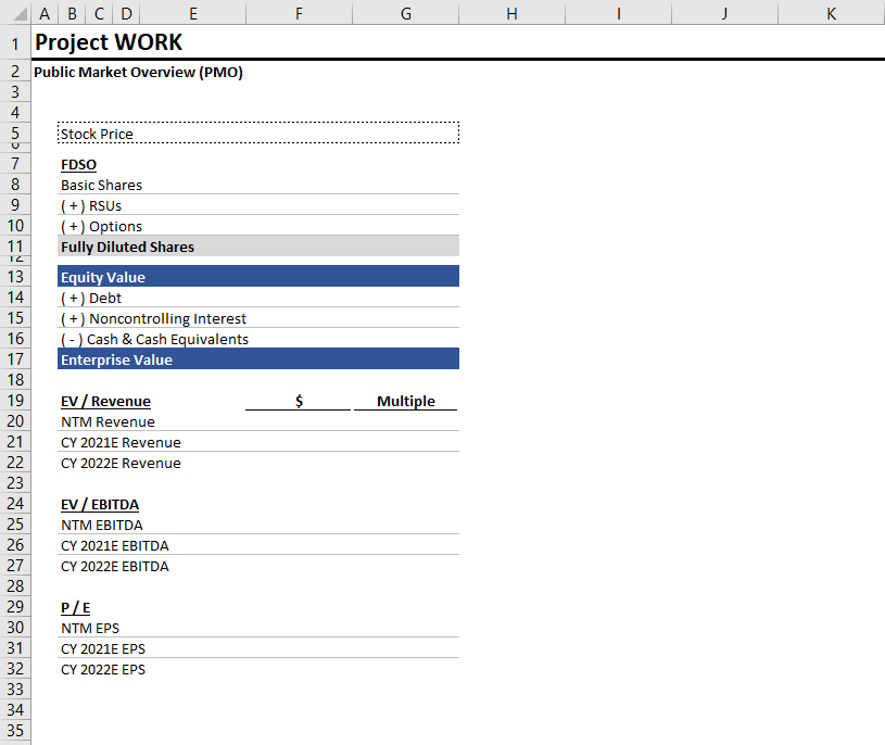
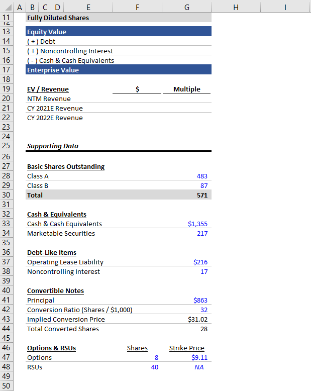
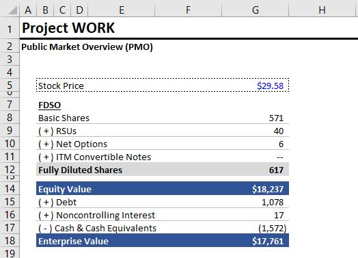
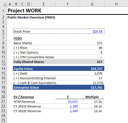
In our prior article, we introduced public filings research and showed you how to calculate enterprise value and implied trading multiples. Together, we built a Public Market Overview (PMO) for Slack.
Now, we’re going to explain the art of parsing a public company’s filings in order to model the company’s future performance. Each company’s financials form a unique puzzle, and deciding which line items to focus on requires significant judgment. Furthermore, many companies’ disclosures are inconsistent over time (as we will see with Slack).
This article will guide you through Slack’s historical financials. We will show you how to weigh which data points to include, and which to ignore. We will also detail the process for collecting cleaned quarterly data, which will be the input for our next article on building operating cases. A model without clean data is an exercise in futility.
High-Level Discussion
It’s natural to start a modeling project by diving into financial statements and entering numbers in Excel. I’m guilty of that myself. Guilty!? Isn’t that what you’re supposed to do? Well, yes, but let’s take a minute to map things out and discuss what we’re looking for first.
If you think about it, financial statements are actually an output. We read them and perform analyses in order to draw inferences from the data. Does the given company have strong cash flow? How are its unit economics trending? We take the financial statements, the output, and we try to better understand the machine that produced them, the company.
Financial modeling, when done right, should normalize this order of operations. We model the drivers of the business, and the resulting financial statements are once again an output. So how do we find and model the key drivers for a business?
Building an Operating Model
That question is the crux of building an operating model. The first step is familiarizing yourself, at a high-level, with the given company and its business model.
If you’re unfamiliar with a public company, or its business model, skimming its latest 10-K is a great place to start. Here’s Slack’s latest 10-K.
Once you know the basics, the next step is identifying the key metrics for that business model. What information / line items would you need in order to make an illustrative income statement? You definitely need to know revenue drivers, preferably unit prices and volumes. Likewise, you need to understand the cost structure, CapEx requirements, and working capital.
Applying this framework to Slack, let’s start by identifying Slack’s business model. Slack is a Software-as-a-Service (SaaS) company. SaaS businesses make money by charging customers monthly, quarterly, annual, or multi-year subscriptions. You can break down a SaaS business’ revenue model into several variables:
- Number of customers
- Average subscription ($) per customer
- Average churn (percentage of customers that leave over a given time period, e.g., monthly churn)
- Number of projected new customers
Ideally, you’d have this historical data by customer segment (the specific customer segments depend on the business) or cohort (dare to dream). But you’re unlikely to find this data for a public company, even in aggregate. You have to make do with what’s available.
On the cost side, SaaS businesses are straightforward:
- Sales costs are a variable expense, since reps get paid commission for new deals and renewals.
- Customer support should be a variable expense (tied to number of customers or revenue).
- Computing infrastructure costs (e.g., AWS) should be relatively fixed / a step function.
- You can think of R&D (product & engineering) as a mix of growth and maintenance CapEx. Most SaaS businesses invest heavily in product, especially in the early years. To be conservative, we can model R&D as a variable cost.
- Marketing is also a variable expense, but it’s a weird one, because marketing dollars spent today will earn money far into the future (hello, subscription revenue). Marketing expenses should be connected to customer growth (more marketing dollars = more new deals).
- Lastly, G&A is somewhat of a step function, but can be modeled conservatively as a variable cost.
Just like on the revenue side, we’ll have to make do with what’s available. We won’t get everything. But now you should have a clearer understanding of the operating drivers we’re looking for.
Fixed vs. Variable Costs
You probably already know the distinction, but it’s worth covering just in case. Fixed costs are costs that do not change as a function of sales in the near-term. For example, you probably won’t get a new office if you sell 5 more units tomorrow. The office rent expense is a fixed cost.Variable expenses, well, vary with revenue. For example, you sell pencils. If you sell more pencils, you will spend more money on wood and graphite (inputs) and labor (to make pencils). These are variable costs.
Summary
So far, we’ve:
- Identified Slack’s business model, Software-as-a-Service (SaaS).
- Discussed key revenue and cost drivers.
Now, we’re going to:
- Comb through Slack’s financials to assess what data is available.
- Pull and clean Slack’s historical data.
Assessing What Data’s Available
We’ve discussed the metrics on our wish list. Now, we need to assess what’s actually available. To that end, I recommend the following:
- Read the latest 10-Q.
- Skim the latest 10-K. Here the focus is on surveying what’s included rather than reading the content.
- Read the latest earnings release. This is the Exhibit 99.1 that’s included as part of the 8-K immediately preceding a 10-Q/10-K. (If a company releases multiple 8-Ks on the same day, you may need to click on several to find the earnings release.) The earnings release is usually where management discloses non-GAAP metrics.
- Check the prior earnings release to confirm it’s consistent with the latest one (sometimes companies are inconsistent).
The good and the bad news is that Slack doesn’t provide much besides the mandatory disclosures. That’s good, because it means less work, and it’s bad, because it means we have less operating data for building projections.
Price / Volume Data
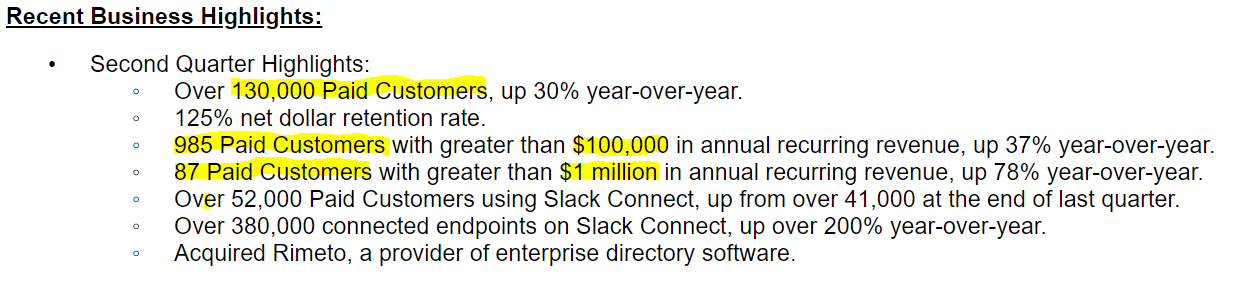
In the latest earnings release, Slack provides the following data points:
- Number of customers (total)
- Number of customers paying $100,000+ annually
- Number of customers paying $1,000,000+ annually
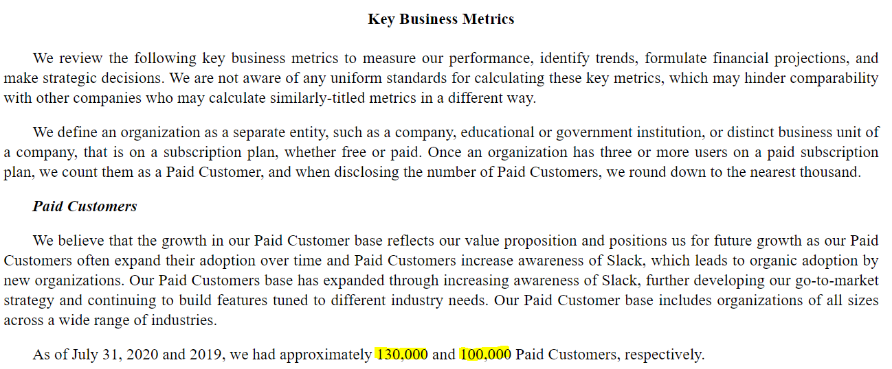
Likewise, in the 10-Q, Slack offers a couple additional nuggets. First, under Management’s Discussion and Analysis (MD&A), there’s a section titled “Key Business Metrics,” which reiterates the customer counts.
Customer Pricing
More importantly, the Key Business Metrics section of the 10-Q includes the percentage of revenue allocated to customers paying $100,000+. Therefore, we also know the percentage of revenue contributed by all other customers (those paying less than $100,000 annually).

This data point is crucial, because the customer counts alone do not enable us to create a detailed revenue build. Now that we have the percentage of revenue by customer segment, however, we can calculate the revenue per segment (segment percentage x total revenue). Then we can divide the revenue per segment by the segment customer count in order to derive the average revenue per customer. This is essentially the unit price, so we have price / volume data by segment for a detailed revenue build.
Since Slack doesn’t disclose the percentage of revenue from $1,000,000+ customers, we’ll ignore them. Instead, we’ll focus on two segments: large customers ($100,000+) and everyone else. Anyways, $1,000,000+ customers are implicitly bundled as part of the $100,000+ segment.
Quick aside - it’s fascinating seeing how much of Slack’s revenue (~50%) comes from its biggest customers. This is a key diligence area:
- Can Slack continue converting smaller customers into big customers?
- How well does Slack retain its largest customers?
- Has Slack lost any big customers?
- What do Slack’s largest customers have to say about the product?
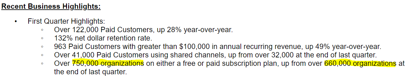
Free Users
In addition to customer counts, the prior earnings release also includes the total number of organizations using Slack (free and paying). Since we know the number of customers, we can deduce the number of free organizations, which is important, because Slack has a freemium sales model. Organizations can begin using the product, and proving value, for free. At a certain point, they reach a paywall and must convert to paying customers. Therefore, the pool of free organizations forms Slack’s supply of potential customers.
When projecting Slack’s revenue, we’ll need to think carefully about the number of free organizations using Slack and what percentage we expect to ultimately convert to paying customers.
Customer Retention / Churn
You may have noticed that Slack also discloses a Net Dollar Retention Rate.
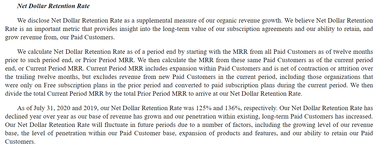
It took us a few reads to understand what this metric represents. Basically, for any period, Slack looks at its customers a year prior and compares the revenue from that group a year ago to the revenue from that group today. This metric ignores new customers (won in the past year) in order to measure the aggregate impact of:
- Churned customers
- Existing contract increases
- Existing contract decreases
Ideally, we would like to include this metric as part of our revenue build, but unfortunately, it combines too many separate variables. We also have no knowledge of its breakdown by customer segment. Therefore, we’re not going to focus on net dollar retention when building our operating model, but it is a metric an investor would want to watch.
Cost Data
On the cost side, Slack’s disclosures are pretty light. Hosting costs are the one detail we can glean from the 10-Q notes:
As we discussed above, hosting costs are relatively fixed, but follow a step function. The contract minimums should serve as a good proxy for future costs. Also, in the income statement, hosting costs are contained almost entirely within the cost of revenue line. This enables us to disaggregate hosting costs from the cost of revenue, and we’ll assume the remaining cost of revenue consists of variable support costs.
The 10-Q notes also contain office lease commitments. But unfortunately, rent expense is allocated among several income statement line items. Therefore, it’s impossible to disaggregate, and doing so would add little value.
We’ll pull all other cost data from the income statement.
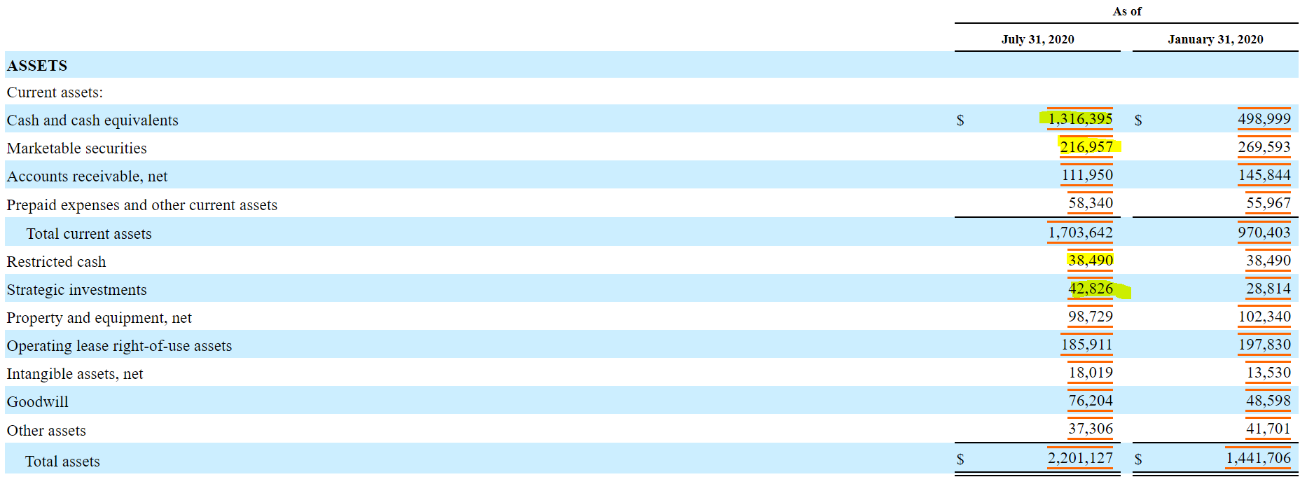
CapEx and Working Capital
Likewise, we’ll find CapEx in the statement of cash flows, and we’ll pull working capital directly from the balance sheet.
1) Starting in Excel
Enough chitchat - let’s start pulling & cleaning some data.
We’re going to start with the final Excel file from our prior article.
And here’s our updated Excel file containing Slack’s cleaned historical financials and operating data. Even if you don’t want to go through this exercise manually, we recommend you skim the guide / discussion below.
Note on Data Scrubbing
Personally, I find pulling and cleaning data extremely tedious, but going through the process always unearths some nuggets. Yes, using a third party data service is faster. It’s less boring. For most use cases, it’s probably accurate enough. But going through the financials yourself means you’re less likely to miss crucial details, and you’ll know the company and its disclosures better.
2) Add New Data Tab
First, we’re going to create a new tab, where we’ll record Slack’s historical data.
- Create a new tab. The shortcut to create a new Excel tab is SHIFT + F11.
- Let’s rename the new tab
Historicals. The shortcut to rename an Excel tab is: ALT > H > O > R. - Let’s apply some basic formatting to the tab. In the upper leftmost cell, we’ll reference the project name.
= “Project “&PROJECT
- Below the project name, let’s put a page header - in this case, “Historical Financial Data”
Your new tab should look like this:
3) Add Dates
Now we’re going to add dates to the tab so we can begin recording Slack’s historical data.
When building a quarterly model, you want at least 2 - 3 years of historical data, so that you can see trends emerge over the course of each year. Slack’s business shouldn’t have much seasonality, but its working capital may fluctuate by quarter.
Also, we’re building this model from the perspective of a public markets investor prior to Slack’s announced sale to Salesforce. Therefore, we will only look at filings available before November 25, 2020.
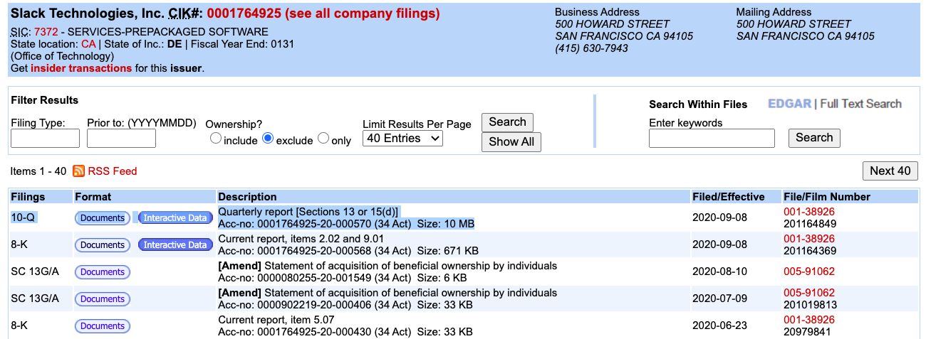
- Let’s return to the SEC EDGAR website. I never remember the URL, so I always google “SEC EDGAR”; the first Google result is correct.
- Where it says Company and Person Lookup, type in WORK (Slack’s ticker). You should see Slack Technologies, Inc. as the first returned option. Here’s the link to Slack’s EDGAR page just in case.
- Scroll through the list of filings until you see ones that were published before November 25, 2020. (Depending on when you’re working through this tutorial, you may have to go back a couple of pages.)
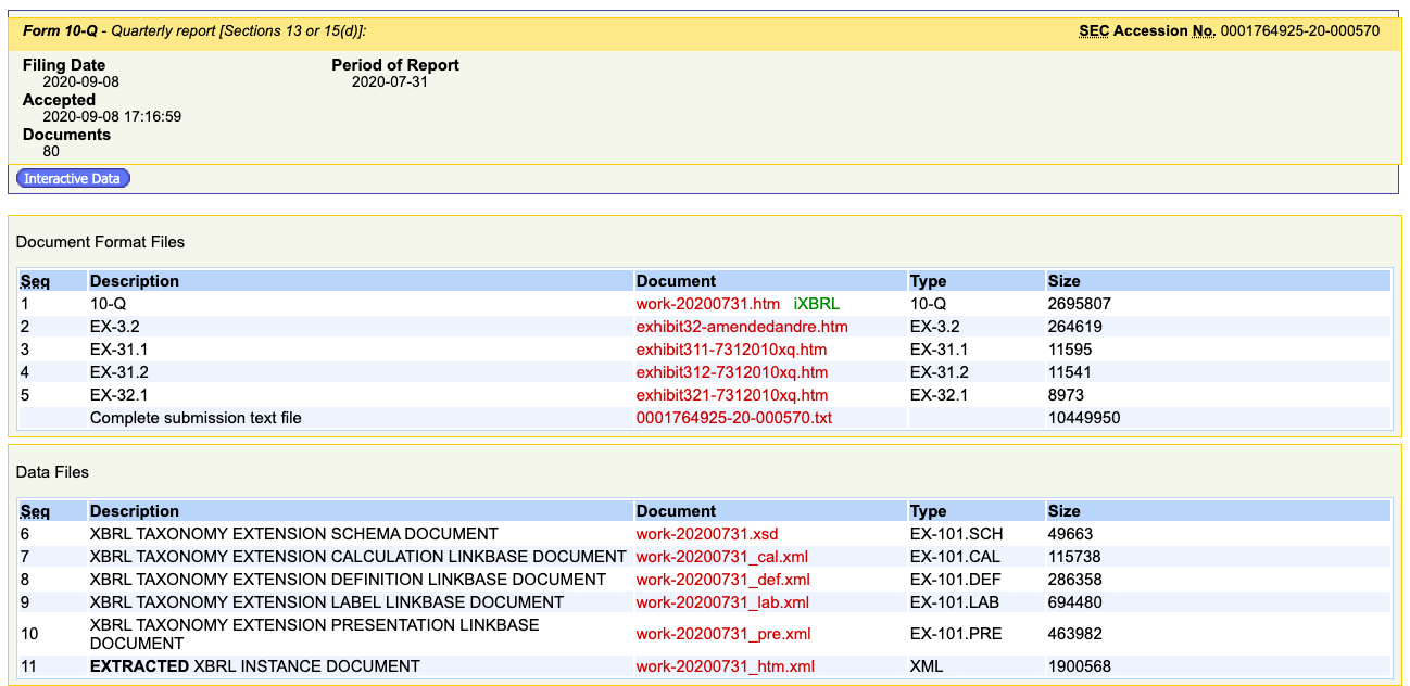
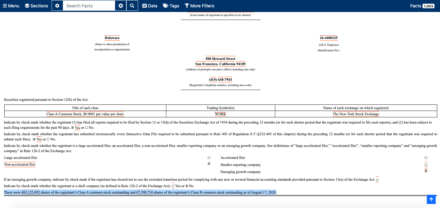
- The last filing before November 25, 2020 is Slack’s 10-Q for Q2 2021. Let’s open that up.
- Scrolling down you should reach the balance sheet pretty quickly. In 10-Q filings, the balance sheet displays account balances for the current quarter and the latest fiscal year end. Therefore, we now know the Q2 date (July 31) and the Q4 date (January 31).

- From these two dates we can extrapolate the remaining quarterly dates. Q1 is April 30; Q3 is October 31. You can double check these.
- Now, in Excel, let’s enter the quarterly dates for the two most recent quarters (Q1 & Q2 2021) and the three preceding fiscal years (2018, 2019, and 2020).
- Your Historicals tab should look like this:
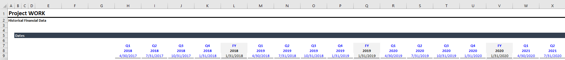
A couple notes:
- We’re entering the dates as a separate section so that we don’t repeat ourselves. Each subsequent section that needs date labels (e.g., the income statement), can link to this date section. It’s best not to hardcode multiple copies of the same information, even simple stuff, like dates.
- We’re including columns for the fiscal years, because some of the data we record may only be available on an annual basis. Also, we will use annual data (from a 10-K) to calculate Q4 quarterly data. Therefore, whenever you’re pulling historical data, you should leave space for annual as well as quarterly columns. You need both.
4) Outline Sections
Let’s outline the sections we’ll be adding to our historical data tab.
Let’s add a blue header row and date rows for each of the following sections:
- Revenue Build
- Income Statement
- Balance Sheet
- Statement of Cash Flows
We’ll also add blue header rows (but not dates) for:
- PP&E
- Intangibles
- Hosting Commitments
We’ll pull PP&E, intangibles, and hosting commitments details from the latest 10-Q.
Before moving on, let’s discuss the notes found in the latest 10-Q, and why we decided to include or skip them.
1) Accounting Policies - for reference only.
2) Revenue & Contract Costs - already covered in the income statement and balance sheet. Also, we’ve decided to focus on customer segments for our revenue build instead of a geographic breakdown.
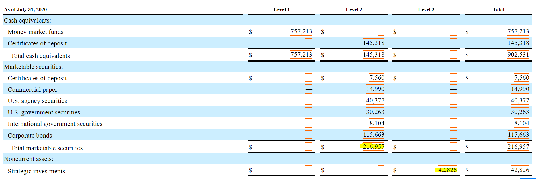
3) Fair Value Measurements - we used this in our PMO, but it’s not particularly relevant to our operating model.
4) Business Combination - the acquired company is already incorporated in the consolidated financials, as we discussed in the prior article.
5) Balance Sheet Components - we will use the PP&E and intangibles data.
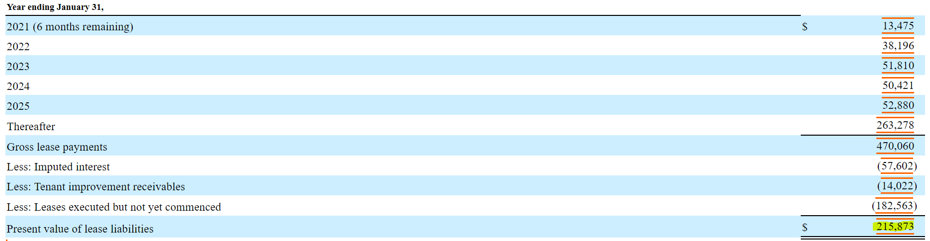
6) Operating Leases - it’s impossible to disaggregate rent expense from the income statement, and it’s not an important variable for a growing SaaS business.
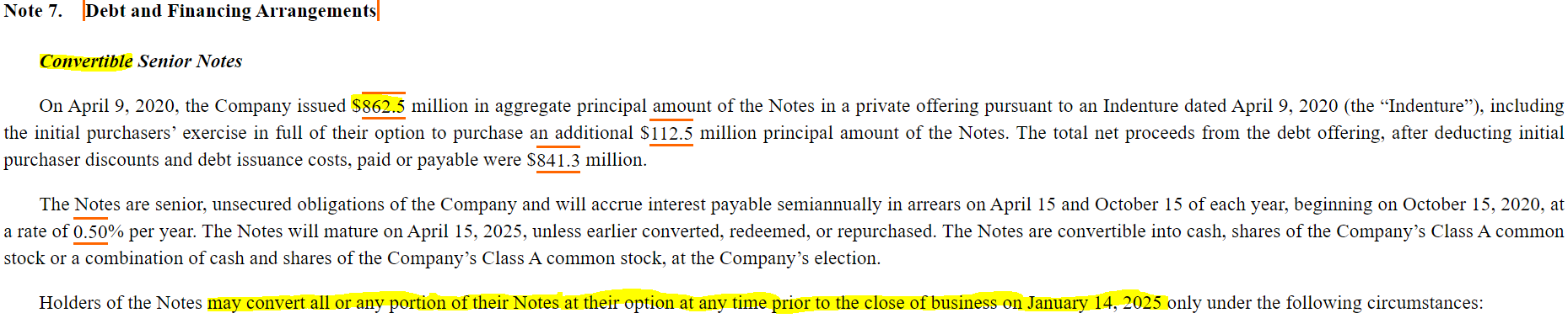
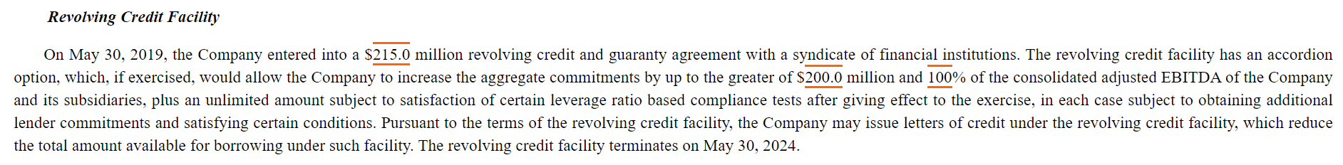
7) Debt & Financing Arrangements - we used the convertibles notes data in our PMO, but it’s financing rather than operating data. To be clear, we’ll need to model the debt in our standalone model, but it’s not something we’ll build an operating case for, so we can leave it out for now.
8) Commitments and Contingencies - as noted, we’re using the hosting commitments data.
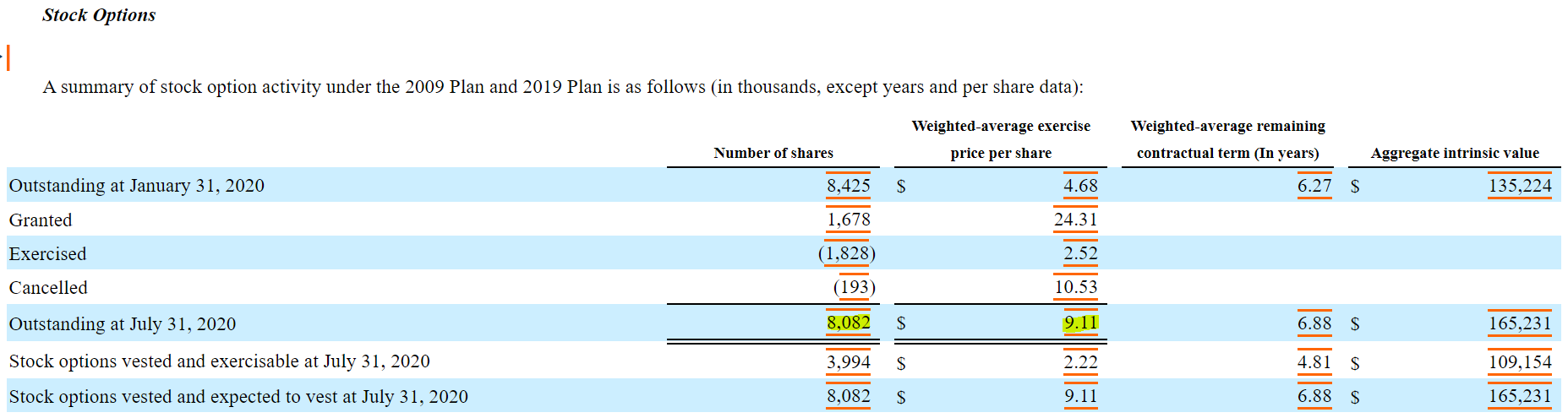
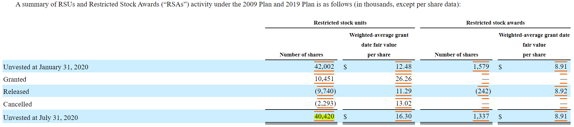
9) Stockholders’ Equity - we used the share awards information in our PMO, but don’t need the rest here.
10) Interest Income and Other Income - we will want to add this detail as part of the income statement section. You can add it as a memo underneath the meat of the income statement.
11) Income Taxes - this is interesting. Slack has a substantial NOL balance, but doesn’t expect to realize any of the value, i.e., the company plans to invest aggressively in growth and anticipates little taxable income. Growth-stage SaaS businesses, like Slack, trade based on revenue, so we can ignore taxes for now.
12) Net Loss Per Share - Slack doesn’t trade based on EPS, so who cares.
5) PP&E & Intangibles
We’re pulling the latest PP&E and intangibles data so that we can build detailed depreciation and amortization schedules. Public markets investors pay attention to SaaS businesses’ cash flow generation, and D&A is an important part of free cash flow.
Fortunately, it is very easy to get this data - we can pull it directly from the latest 10-Q.
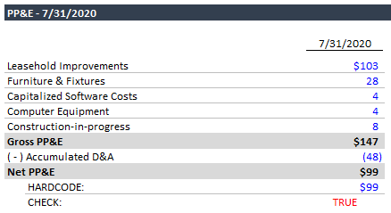
PP&E
Here’s the relevant section in the 10-Q:
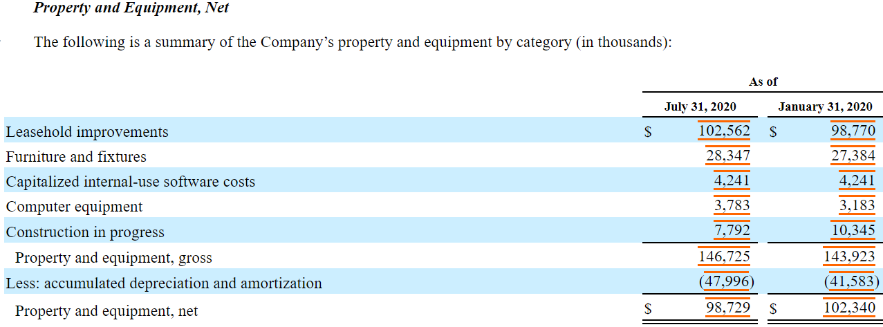
And here’s our transcribed data in Excel:
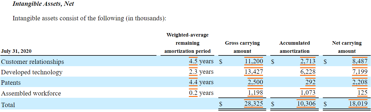
Intangibles
Here’s the relevant section in the 10-Q:
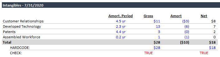
And here’s our transcribed data in Excel:
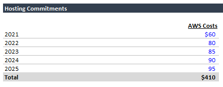
6) Hosting Commitments
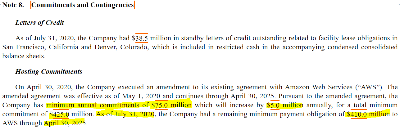
Similarly, we can find hosting commitments in the latest 10-Q. Here’s the relevant section:
From this blurb, we learn the following:
- Slack has already spent $15 million on hosting this year ($425 - $410).
- Slack must spend at least $60 million on hosting during Q3 and Q4 this year ($75 - $15).
- Next year (FY 2022), Slack has a minimum AWS hosting commitment of $80 million. In FY 2023, Slack must spend $85 million on hosting, etc.
- The minimum increases by $5 million each year.
We’re going to use these commitments as our projected hosting costs. Here’s the data in Excel:
7) Income Statement
Next, we’re going to fill in the income statement, copying Slack’s line items exactly.
Note on Process
When gathering financial data, you should always start with the most recent filings and work backwards, because the latest filings are the most up-to-date. Let’s look at an example.You’re modeling ABC Company, which just released a 10-Q. During this past quarter, ABC Company acquired XYZ LLC, and the 10-Q financial statements include the impact of the deal. Even the financials for the prior year include XYZ LLC, since the financials are consolidated.
If you look at the prior year’s 10-Q, however, that 10-Q does not include the impact of the deal (since the deal hadn’t happened yet).
Therefore, you should pull as much data as possible from the latest filings, and you can fill in the gaps working backwards.
Let’s apply this process to the income statement:
- We’ll start with the latest 10-Q, which includes data for Q2 2021 and Q2 2020.
- Likewise, the prior 10-Q includes data for Q1 2021 and Q1 2020.
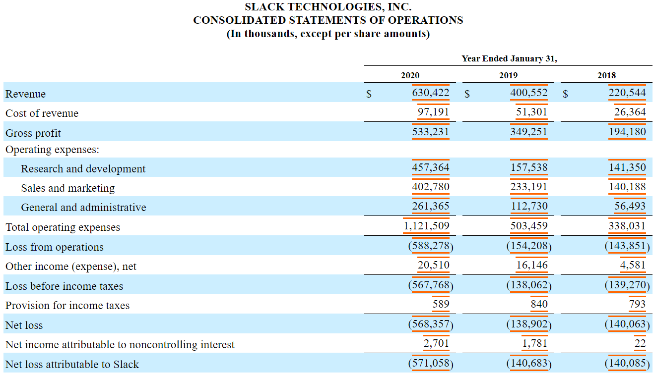
- Working backwards, next we need quarterly data for Q4 2020. But – the plot thickens – there is no 10-Q for Q4. Instead we have the 10-K, which provides annual financials for FY 2020, FY 2019, and FY 2018. Save the annual data under the fiscal year columns. Here’s the annual income statement:
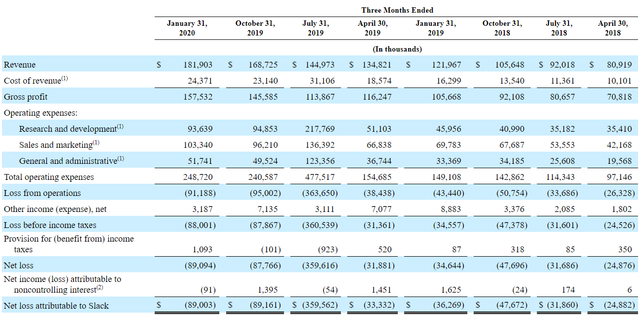
- In addition to annual data, the 10-K also has a quarterly income statement for the preceding two years (FY 2019 and FY 2020). To find it, open the 10-K and search “quarterly results of operations.” This quarterly data extends beyond the oldest available 10-Q (Q2 2020), so we’ve captured all of the core income statement data that we have access to. Here’s the quarterly income statement from the 10-K:
Here’s what our updated income statement section looks like in Excel:
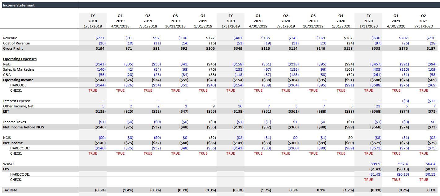
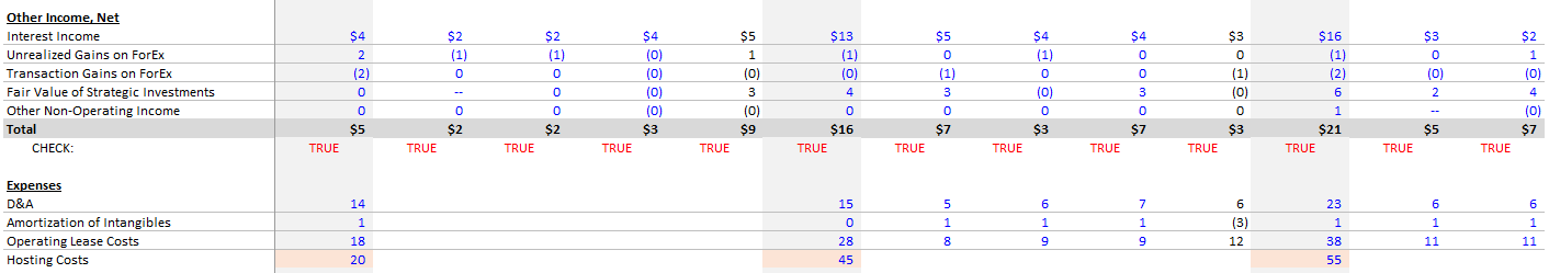
You’ll notice we included the breakdown of other income and a few extra line items. The cells shaded pink / orange are estimates.
8) Revenue Build
Now that we have historical revenue, we can turn to our revenue build. We need to pull the following data points for each time period:
- Customer count
- $100,000+ customer count
- Free organizations count (they use Slack but don’t pay)
- Percentage of revenue from customers paying $100,000+ annually
A few notes before you get started:
- As we saw with the two most recent earnings releases (one had the free organization count, and the other did not), you won’t be able to find every data point for each period. Sometimes, the data is missing. That’s okay - we’ll work with what we have.
- These data points, particularly the percentage of revenue, are often buried in paragraphs of text. Ctrl + F is your friend.
- Word to the wise: Find the data points for the first couple quarters manually. Learn the words that Slack uses to describe / surround these metrics, and then search through the older filings using these keywords.
After lots of searching, you should have the following data:

We couldn’t find data for the cells shaded pink / orange, but we added estimates to some of them.
Deriving Unit Pricing & Volumes
Between the metrics above and historical revenue (from the income statement), we should be able to derive the following:
- Revenue per big customer ($100,000+)
- Revenue per small customer (< $100,000)
Take a minute, and try to figure out how you would calculate these values using the information available.
Okay, need a hint? Here are the rows from our revenue build:
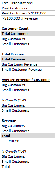
Try to fill in those rows with the correct formulas. If you’re stuck, check out the completed Excel file.
Ultimately, this is what your revenue build section should look like:
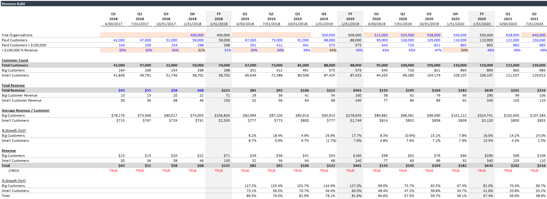
At first glance, the numbers look good. Slack’s revenue per customer increased (YoY) almost every quarter. The revenue per customer for big customers looks particularly juicy. You could interpret this in several ways:
- Slack grows within its largest accounts like a virus.
- Slack’s larger, but-still-small customers are growing rapidly, and Slack grows with them. They eventually convert from small to big.
- Slack is landing bigger and bigger fish.
The truth is probably a mix of all three (and some other options we’re not thinking of).
9) Balance Sheet
The balance sheet is straightforward, but extra tedious. It’s extra tedious, because each 10-Q contains balance sheet data for the current quarter and the prior fiscal year end. This means that the Q1 and Q2 10-Qs only contain balance sheet data for three quarters combined (since both reference the same prior fiscal year end).
Alas, let’s throw on some tunes and grind it out.
At a certain point we ran out of historical data, so our balance sheet looks a bit abbreviated compared to the income statement. Here it is:
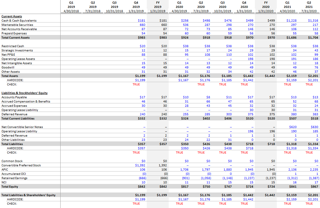
Pro Tip: Use Footnotes
We were lazy and didn’t add footnotes to our historical data. Don’t do that. At the very least, each hard-coded number should include the URL for the relevant filing. That way, if you need to find the source, you can pop open the relevant filing and Ctrl + F for the number.
Aside: On Balance Sheets
When building standalone models, a lot of people skip the balance sheet or simplify it. If you’re working on high-level banker outputs, sure, I get it. But if you’re an investor, use the real thing. Learn what each line item represents. As an investor, it’s important to monitor the balance sheet and think critically about what’s being capitalized and whether it’s appropriate.
10) Statement of Cash Flows
Last but not least, we need the statement of cash flows. We’re actually going to split this into two sections due to a reporting complication: 10-Qs show cash flow data on a cumulative basis. This means Q1 contains the cash flows for the three months of Q1. But Q2 contains combined cash flows for Q1 + Q2, and Q3 contains cash flows for Q1 + Q2 + Q3.
To remedy this, and calculate a quarterly statement of cash flows, we need two copies of the statement of cash flows. The first copy will consist of the data as reported. The next copy will be our quarterly output. Once we have the raw data, calculating the quarterly figures is straightforward:
- Q1 calculated = Q1 as reported.
- Q2 calculated = Q2 as reported - Q1 as reported.
- Q3 calculated = Q3 as reported - Q2 as reported.
- Q4 calculated = Annual as reported - Q3 as reported.
Now that you know the workflow, let’s throw on some tunes and get going.
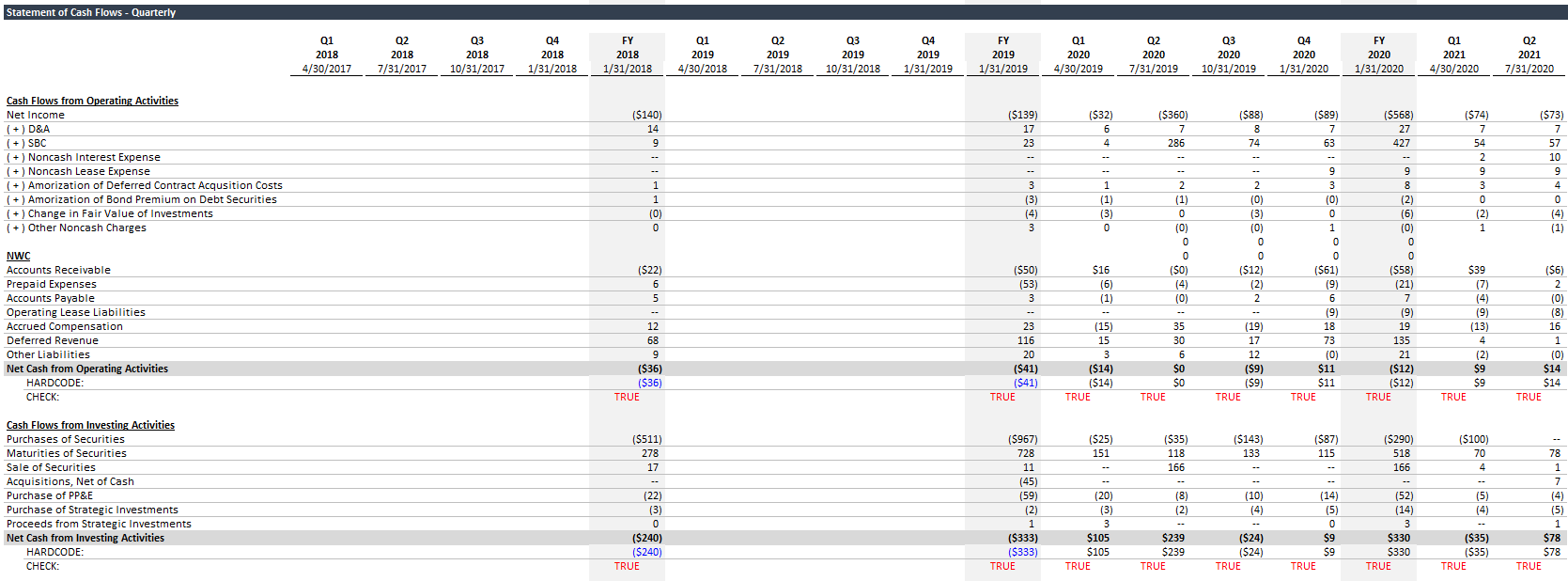
Here’s the statement of cash flows as reported:
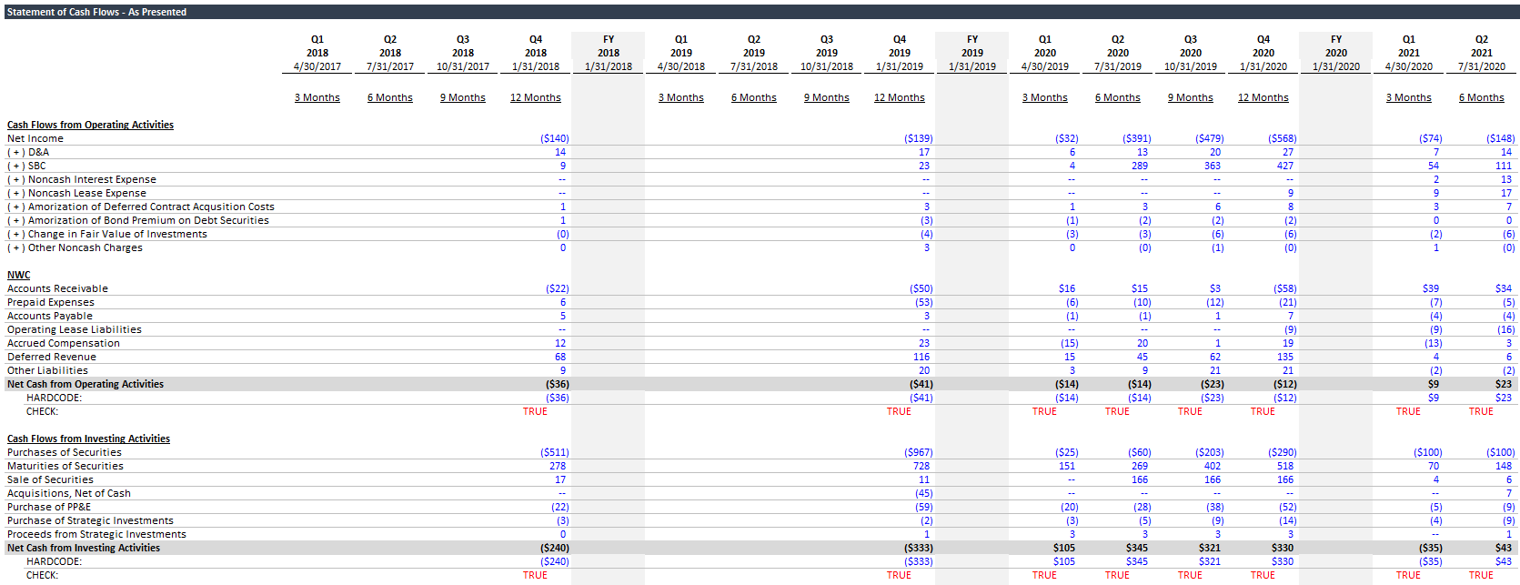
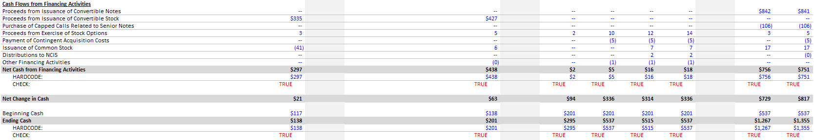
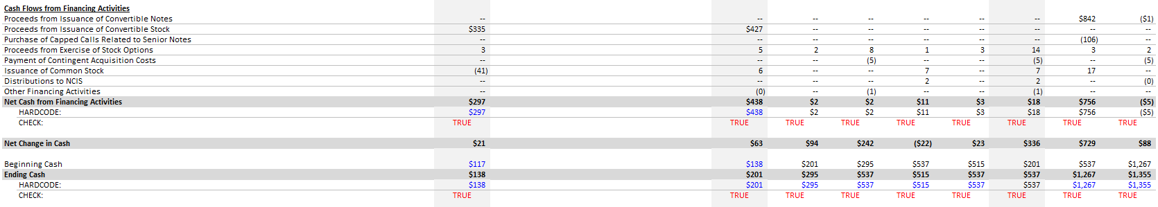
And here’s the quarterly statement of cash flows:
Pro Tip: Working Capital Comparison
In our standalone model, we’ll be projecting working capital using balance sheet / income statement ratios (e.g., Days Sales Outstanding). We’ll derive these ratios by comparing historical income statement and balance sheet data.You should always compare balance sheet working capital changes to values reported in the statement of cash flows. Why? Because if the numbers aren’t close, that means the company is stuffing other items into the working capital lines in the statement of cash flows. Therefore, your projections won’t capture the stuffed items (because you’re using balance sheet and income statement data for the projections), and your projected line items won’t really be comparable to the historical values. This is nightmare fuel for a financial analyst, and there’s not an easy remedy.
Fortunately, we checked, and Slack’s balance sheet changes at least approximate the values reported in the statement of cash flows. Nice job, Slack! Feel free to compare the two and check for yourself:
- Beneath your quarterly statement of cash flows, add some placeholder lines for the balance sheet working capital changes.
- In that space, calculate the changes in balance sheet working capital lines quarter-by-quarter. For example, the change in Net Accounts Receivable = beginning period Net AR - ending period Net AR. If net accounts receivable increases, that’s cash you didn’t receive this quarter, so it’s effectively a use of cash.
- Compare the calculated balance sheet changes to the values in your quarterly statement of cash flows. As long as they’re close, that means we’re on the right track.
- You should also be careful to add any related items when comparing the two. For example, if the statement of cash flows separately reports bad debt expense, that line should be added to the accounts receivable line for the comparison, since the balance sheet reports accounts receivable net of the allowance for doubtful accounts.
- Once you’ve checked that the working capital values roughly match, go ahead and delete the comparison calculations. They won’t be need anymore.
Conclusion
Congrats! It was a slog, but we’ve pulled Slack’s historical data, and we’re ready for the next step: building operating cases. Soon, we’ll have our standalone model.
In this tutorial, you:
- Continued exploring the SEC EDGAR website
- Learned how to pull historical financial data
- Became more familiar with financial footnotes
- Learned the framework for targeting your data search – what’s the company’s business model, and what key metrics do I need?
Reach out with any questions.


")
